CHEM E 310 Material and Energy Balances
Contents
Units and Process Variables
Force
| Description | Equations |
|---|---|
| Units of force | $\begin{aligned}1 \ \mathrm{N} &= 1 \ \mathrm{kg \cdot m/s^2} \cr 1 \ \mathrm{lb_f} &= 32.174 \ \mathrm{lb_m \cdot ft/s^2}\end{aligned}$ |
| Weight | $W = mg$ |
| Gravitational acceleration | $\begin{aligned}g &= 9.8066 \ \mathrm{m/s^2} \cr &= 32.174 \ \mathrm{ft/s^2}\end{aligned}$ |
Mass, volume and flow rate
| Description | Equations |
|---|---|
| Mass flow rate | $\dot{m} = \dfrac{dm}{dt}$ |
| Volumetric flow rate | $\dot{V} = \dfrac{dV}{dt}$ |
| Molar flow rate | $\dot{n} = \dfrac{dn}{dt}$ |
| Density | $\rho = \dfrac{m}{V} = \dfrac{\dot{m}}{\dot{V}}$ |
| Specific volume | $v = \dfrac{V}{m} = \dfrac{1}{\rho}$ |
| Molar volume | $V_{\mathrm{m}} = \dfrac{V}{n} = \dfrac{M}{\rho}$ |
| Specific gravity | $\mathrm{SG} = \dfrac{\rho}{\rho_{\mathrm{ref}}}$ |
Chemical composition
| Description | Equations |
|---|---|
| Mole and molecular wieght | $n = \dfrac{m}{M}$ |
| Mass fraction | $x_A = \dfrac{m_A}{m}$ |
| Mole fraction | $y_A = \dfrac{n_A}{n}$ |
| Scaling factor of percent (%), parts per million (ppm), parts per billion (ppb) |
$\times 100\% \newline \times 10^6 \ \mathrm{ppm} \newline \times 10^9 \ \mathrm{ppb}$ |
| Average molecular weight | $\overline{M} = \dfrac{\sum m_i}{\sum n_i} = \sum y_i M_i = \left(\sum\dfrac{x_1}{M_i}\right)^{-1}$ |
| Mass concentration | $\rho_A = \dfrac{m_A}{V}$ |
| Molar concentration | $c_A = \dfrac{n_A}{V}$ |
| Molarity and molar | $1 \ \mathrm{M} = 1 \ \mathrm{mol}/\mathrm{L}$ |
Pressure
| Description | Equations |
|---|---|
| Pressure | $P = \dfrac{F}{A}$ |
| Hydrostatic pressure | $P = P_0 + \rho gh$ |
| Hydrostatic head | $P = \rho gP_h$ |
| Relationship between pressures | $P_{\text{abs}} = P_{\text{atm}} + P_{\text{gauge}}$ |
| General manometer | $P_1 + \rho_1 g d_1 = P_2 + \rho_2 g d_a + \rho_m g h$ |
| Differential manometer | $P_1 - P_2 = (\rho_m - \rho)gh$ |
| Manometer for gas | $P_1 - P_2 = \rho_m gh = P_h$ |
| SCFM (standard cubic feet per minute) and ACFM (actual cubic feet per minute) | $\dot{V_{\text{a}}} = \dot{V_{\text{s}}}\dfrac{P_{\text{s}}}{P_{\text{a}}} \dfrac{T_{\text{a}}}{T_{\text{s}}} \ (\text{ideal gas})$ |
| Standard condition of gases | natural gas - $59 ^\circ\mathrm{F}, 1 \ \mathrm{atm}$ other gas - $0 ^\circ\mathrm{C}, 1 \ \mathrm{atm}$ |
Temperature
| Description | Equations |
|---|---|
| Conversion of temperature | $T(\mathrm{K}) = T(\mathrm{^\circ C}) + 273.15 \newline T(\mathrm{^\circ R}) = T(\mathrm{^\circ F}) + 459.67 \newline T(\mathrm{^\circ R}) = 1.8 T(\mathrm{K}) \newline T(\mathrm{^\circ F}) = 1.8 T(\mathrm{^\circ C}) + 32$ |
| Conversion of temperature intervals | $1 ^\circ\mathrm{C} = 1.8 ^\circ\mathrm{F} \newline 1 ^\circ\mathrm{R} = 1.8 \ \mathrm{K} \newline 1 ^\circ\mathrm{F} = 1 ^\circ\mathrm{R} \newline 1 ^\circ\mathrm{C} = 1.8 \ \mathrm{K}$ |
Fundamentals of Material Balances
Concepts
| Description | Equations |
|---|---|
| Balance equation | Accumulation = Input - Output + Generation - Consumption |
| Fractional excess | $\text{Fractional excess} = \dfrac{n_{\mathrm{fed}} - n_{\mathrm{stoich}}}{n_{\mathrm{stoich}}}$ |
| Fractional conversion | $\text{Fractional conversion} = \dfrac{n_{\mathrm{reacted}}}{n_{\mathrm{fed}}}$ |
| Fractional completion of limiting reactant | $\text{Fractional completion} = \dfrac{n_{\mathrm{reacted}}}{n_{\mathrm{fed}}} = \dfrac{-\nu\xi}{n_{\mathrm{fed}}}$ |
| Extent of reaction | $\xi = \dfrac{n_i - n_{i0}}{\nu_i}$ |
| Extent of reaction in multiple reactions | $n_i = n_{i0}\sum\limits_j\nu_{ij}\xi_{ij}$ |
| Yield theoretical = complete rxn, no side rxn |
$\text{Yield} = \dfrac{n_\text{actual}}{n_\text{theoretical}} \times 100%$ |
| Selectivity | $\text{Selectivity} = \dfrac{n_\text{desired}}{n_\text{undesired}}$ |
| Fractional excess of air (oxygen) | $\text{Fractional excess air} = \dfrac{n_{\mathrm{fed}} - n_{\mathrm{stoich}}}{n_{\mathrm{stoich}}}$ |
| Quality of steam | $\text{Quality of steam} = \dfrac{m_{\text{vapor}}}{m_{\text{total}}}$ |
Degree of freedom analysis
| Description | Equations |
|---|---|
| Nonreactive process | $\small\begin{aligned} & \text{No. unknown variables} \cr - & \text{No. independent material balance species} \cr - & \text{No. other relations (process specifications)} \cr \hline & \text{No. degrees of freedom}\end{aligned}$ |
| Reactive process Molecular species balance method 1 reaction system |
$\small\begin{aligned} & \text{No. unknown variables} \cr + & \text{No. independent reaction} \cr - & \text{No. independent molecular species} \cr - & \text{No. other relations} \cr \hline & \text{No. degrees of freedom}\end{aligned}$ |
| Reactive process Atomic species balance method >1 reaction system |
$\small\begin{aligned} & \text{No. unknown variables} \cr - & \text{No. independent reactive atomic species} \cr - & \text{No. independent nonreactive molecular species} \cr - & \text{No. other relations} \cr \hline & \text{No. degrees of freedom}\end{aligned}$ |
| Reactive process Extent of reaction method equilibrium problem |
$\small\begin{aligned} & \text{No. unknown variables} \cr + & \text{No. independent reaction} \cr - & \text{No. independent reactive species} \cr - & \text{No. independent nonreactive species} \cr - & \text{No. other relations} \cr \hline & \text{No. degrees of freedom}\end{aligned}$ |
Single-Phase System
Condensed phases
| Description | Equations |
|---|---|
| Estimations of density of liquid mixtures 1. Experimental data 2. Estimation formula ★ Volume addativity |
$\dfrac{1}{\bar{\rho}} = \sum\limits_{i=1}^n \dfrac{x_i}{\rho_i} \newline \bar{\rho} = \sum\limits_{i=1}^n x_i\rho_1$ |
| Incompressible approximation | $\partial\hat{V} = 0 \newline \left(\frac{\partial\hat{V}}{\partial P}\right)_T = 0 \newline \left(\frac{\partial\hat{V}}{\partial T}\right)_P = 0$ |
| Volume expansivity | $\beta = \dfrac{1}{\hat{V}} \left(\dfrac{\partial\hat{V}}{\partial T}\right)_P$ |
| Isothermal compressibility | $K = -\dfrac{1}{\hat{V}} \left(\dfrac{\partial\hat{V}}{\partial P}\right)_T$ |
| Volume with change in $T, P$ | $\ln\left(\dfrac{\hat{V}_2}{\hat{V}_1}\right) = \beta(T_2 - T_1) - K(P_2 - P_1)$ |
Ideal gas of single component
| Description | Equations |
|---|---|
| Specific molar volume | $\hat{V} = \dfrac{V}{n}$ |
| Ideal gas equation of state ★ $\footnotesize T > 0\mathrm{^\circ C}, P < 1 \ \mathrm{atm}$ |
$PV = nRT \newline P\hat{V} = RT$ |
| Standard conditions and actual conditions | $\dfrac{PV}{P_{\text{s}}\hat{V_{\text{s}}}} = n\dfrac{T}{T_{\text{s}}}$ |
| SCFM vs. ACFM ★ Ideal gas |
$\dot{V_{\text{a}}} = \dot{V_{\text{s}}}\dfrac{P_{\text{s}}}{P_{\text{a}}} \dfrac{T_{\text{a}}}{T_{\text{s}}}$ |
| Ideal gas condition | $T > 0 \mathrm{^\circ C} \newline P < 1 \ \mathrm{atm} \newline \footnotesize\hat{V}_{\text{ideal}} = \dfrac{RT}{P} \newline \begin{cases} >5 \ \mathrm{L/mol}, 80 \ \mathrm{ft^3/lbmol} & \text{diatomic} \cr >20 \ \mathrm{L/mol}, 320 \ \mathrm{ft^3/lbmol} & \text{other} \end{cases}$ |
Ideal gas of multiple components
| Description | Equations |
|---|---|
| Partial pressure | $P_i = y_i P$ |
| Dalton’s law | $\sum P_i = P$ |
| Pure-component volume | $V_i = y_i V$ |
| Amagat’s law | $\sum V_i = V$ |
| Volume fraction of ideal gas | $y_i = \dfrac{V_i}{V}$ |
van der Waals equation of state
| Description | Equations |
|---|---|
| van der Waals equation of state | $P = \dfrac{RT}{\hat{V} - b} - \dfrac{a}{\hat{V}^2}$ |
| Constant | $a = \dfrac{27R^2T_c^2}{64P_c}$ |
| Constant | $b = \dfrac{RT_c}{8P_c}$ |
| Significance of 3 real roots | $\hat{V}_{\text{highest}} = \hat{V}_{\text{sat, vapor}} \newline \hat{V}_{\text{lowest}} = \hat{V}_{\text{sat, liquid}} \newline \hat{V}_{\text{middle}} = \small \text{no significance}$ |
| Significance of real and imaginary roots | $\hat{V}_{\text{real}} = \hat{V}_{\text{gas}} \newline \hat{V}_{\text{imaginary}} = \small\text{no significance}$ |
Virial equation of state
| Description | Equations |
|---|---|
| Virial equation of state | $\dfrac{P\hat{V}}{RT} = 1 + \dfrac{B}{\hat{V}} + \dfrac{C}{\hat{V}^2} + \dfrac{D}{\hat{V}^3} + \cdots$ |
| First order appox. of virial equation of state | $\dfrac{P\hat{V}}{RT} = 1 + \dfrac{BP}{RT}$ |
| Reduced temperature | $T_r = \dfrac{T}{T_c}$ |
| Reduced pressure | $P_r = \dfrac{P}{P_c}$ |
Using virial equation of state
- Lookup $T_c, P_c, \omega$
- Calculate $T_r$
- Estimate B by
- $B_0 = 0.083 - \dfrac{0.422}{T_r^{1.6}}$
- $B_1 = 0.139 - \dfrac{0.172}{T_r^{4.2}}$
- $B = \dfrac{RT_c}{P_c}(B_0 + \omega B_1)$
- Substitute known values into first order approximation
Redlick-Kwong (RK) equation of state
| Description | Equations |
|---|---|
| SRK equation of state | $P = \dfrac{RT}{\hat{V} - b} - \dfrac{a}{T^{0.5}\hat{V}(\hat{V}+b)}$ |
| Constants | $a = 0.4274 R^2 T_c^{2.5} / P_c \newline b = 0.08664 RT_c / P_c$ |
Soave-Redlick-Kwong (SRK) equation of state
| Description | Equations |
|---|---|
| SRK equation of state | $P = \dfrac{RT}{\hat{V} - b} - \dfrac{\alpha a}{\hat{V}(\hat{V}+b)}$ |
| Constants | $a = 0.4274 (RT_c)^2 / P_c \newline b = 0.08664 RT_c / P_c \newline m = 0.48508 + 1.55171\omega - 0.1561\omega^2 \newline T_r = T/T_c \newline \alpha = [1 + m(1-\sqrt{T_r})]^2$ |
Using SRK equation of state
- Lookup $T_c, P_c, \omega$
- Calculate $a, b, m$
- Determine the known
- If known $T, \hat{V}$
- Calculate $T_r, \alpha$
- Solve from equation directly for $P$
- If known $T, P$
- Use equation and all knowns
- Use python to solve for $\hat{V}$
- If known $P, \hat{V}$
- Use equation, $T_r, \alpha$, and all knowns
- Use python to solve for $T$
- If known $T, \hat{V}$
Compressibility-factor equation of state
| Description | Equations |
|---|---|
| Compressibility (Law of corresponding state) |
$z = \dfrac{P\hat{V}}{RT}$ |
| Compressibility-factor equation of state | $P\hat{V} = zRT$ |
| Reduced temperature | $T_r = \dfrac{T}{T_c}$ |
| Reduced pressure | $P_r = \dfrac{P}{P_c}$ |
| Ideal reduced volume | $\hat{V}_r^{\text{ideal}} = \dfrac{P_c\hat{V}}{RT_c}$ |
| Kay’s rule of nonideal gas mixtures Pseudocritical temperature |
$T_c' = \sum y_i T_{ci}$ |
| Pseudocritical pressure | $P_c' = \sum y_i P_{ci}$ |
| Pseudoreduced temperature | $T_r' = \dfrac{T}{T_c'}$ |
| Pseudoreduced pressure | $P_r' = \dfrac{P}{P_c'}$ |
| Ideal pseudoreduced volume | $\hat{V}_r^{\text{ideal}} = \dfrac{P_c'\hat{V}}{RT_c'}$ |
Using compressibility-factor equation of state
- Lookup $T_c, P_c$
- If gas is $\ce{H2/He}$, adjust critical constant by Newton’s correlation
- $T_c^a = T_c + 8 \ \mathrm{K}$
- $P_c^a = P_c + 8 \ \mathrm{atm}$
- Calculate reduced value of two known variables from $T_r, P_r, V_r^{\text{ideal}}$
- Use compressibility chart to determine $z$
- Solve for unknowns from equation
Multi-Phase System
Vapor pressure estimations
| Description | Equations |
|---|---|
| Clapeyron equation | $\dfrac{dP^*}{dt} = \dfrac{\Delta \hat{H}_\text{v}}{T}\dfrac{1}{\hat{V_g} - \hat{V_l}}$ |
| Clapeyron equation | $\dfrac{d(\ln P^*)}{d(1/T)} = -\dfrac{\Delta \hat{H}_\text{v}}{R}$ |
| Clausius-Clapeyron equation | $\ln P^* = -\dfrac{\Delta \hat{H}_\text{v}}{RT} + B$ |
| Clausius-Clapeyron equation | $\ln \left(\dfrac{P_2}{P_1}\right) = -\dfrac{\Delta \hat{H}_\text{v}}{nR} \left(\dfrac{1}{T_2}-\dfrac{1}{T_1}\right)$ |
| Antoine equation (Vapor pressure of species) |
$\log_{10}P^* = A - \dfrac{B}{T+C}$ |
Vapor liquid equilibrium (VLE) calculations
| Description | Equations |
|---|---|
| Gibbs phase rule | $\mathcal{F} = 2 + c - \Pi - r$ |
| Total vapor pressure of immiscible liquids | $P = \sum P_i^*$ |
| Raoult’s law ★ Ideal gas and solution, non-dilute $x_A$ |
$P_A = y_AP = x_AP_A^*(T)$ |
| Henry’s law ★ Ideal gas and solution, dilute $x_A$ |
$P_A = y_AP = x_AH_A(T)$ |
| VLE of real gases $\varphi$ - fugacity coefficient $\gamma$ - activity coefficient |
$y_i\varphi_i P = x_i\gamma_i P^*$ |
| Partition coefficient of ideal gas (Raoult’s law) ★ Ideal gas: $\footnotesize\varphi = 1, \gamma = 1$ |
$K_i = \dfrac{y_i}{x_i} = \dfrac{\gamma_i P_{i}^{*}}{\varphi_i P} = \dfrac{P_{i}^{*}}{P}$ |
| Partition coefficient of ideal gas (Henry’s law) ★ Ideal gas, Henry’s law assumptions |
$K_i = \dfrac{H_i}{P}$ |
Saturation and humidity
| Description | Equations |
|---|---|
| Relative saturation/humidity | $s_r = \dfrac{P_A}{P_A^*(T)}\times 100%$ |
| Molal saturation/humidity | $s_m = \dfrac{P_A}{P-P_A}$ |
| Absolute saturation/humidity | $s_a = \dfrac{P_AM_A}{(P-P_A)M_A}$ |
| Percent saturation/humidity | $s_p = \dfrac{s_m}{s_m^*}\times 100 \% \newline = \dfrac{P_A/(P-P_A)}{P_A^*/(P-P_A^*)}\times 100 \%$ |
Bubble and dew point
| Description | Equations |
|---|---|
| Superheated vapor | $P_A = y_AP < P_A^*(T)$ |
| Saturated vapor and dew point | $P_A = y_AP = P_A^*(T_{\text{dp}})$ |
| Degree of superheat | $T - T_{\text{dp}}$ |
| Bubble point temperature of mixture at constant $P$ | $P = \sum x_iP_i^*(T_{\text{bp}})$ |
| Bubble point pressure of mixture at constant $T$ | $P_{\text{bp}} = \sum x_iP_i^*(T)$ |
| Dew point temperature of mixture at constant $P$ | $\sum\dfrac{y_i}{P_i^*(T_{\text{dp}})}= 1$ |
| Dew point pressure of mixture at constant $T$ | $P_{\text{dp}} = \left[ \sum\dfrac{y_i}{P_i^*(T)} \right]^{-1}$ |
Fundamentals of Energy Balances
Closed system balance
| Description | Equations |
|---|---|
| Kinetic energy | $E_k = \frac{1}{2}mv^2$ |
| Potential energy | $E_p = mgz$ |
| Internal energy | $U(T, V)$ |
| Total energy | $E = U + E_k + E_p$ |
| Work | $W = P\Delta V$ |
| Closed system balance | $\Delta U + \Delta E_k + \Delta E_p = Q+W$ |
| $\Delta E_k = 0$ | Not accelerating |
| $\Delta E_p = 0$ | Not changing height |
| $\Delta U = 0$ | No phase change, chemical reaction, temperature change |
| $Q = 0$ | Insulated system; adiabatic; temperature of system and surrounding the same |
| $W = 0$ | No moving parts, radiation, electric current, flow |
Open system balance
| Description | Equations |
|---|---|
| Work | $\dot{W} = \dot{W}_s + \dot{W}_{fl}$ |
| Enthalpy | $H = U+PV$ |
| Specific properties | $\hat{V} = \frac{V}{m}, \hat{V} = \frac{V}{n}$ |
| Open system balance | $\Delta \dot{H} + \Delta \dot{E}_k + \Delta \dot{E}_p = \dot{Q} + \dot{W}_s$ |
| $\Delta E_k = 0$ | No acceleration; linear velocity of all streams the same |
| $\Delta E_p = 0$ | Stream entering and leaving at same height |
| $\dot{Q} = 0$ | Insulated; adiabatic; system and surrounding temperature the same |
| $\dot{W}_s = 0$ | No moving parts |
| Friction loss | $\hat{F} = \Delta\hat{U} - \dfrac{\dot{Q}}{\dot{m}}$ |
| Mechanical energy balance | $\dfrac{\Delta P}{\rho} + \dfrac{\Delta v^2}{2} + g\Delta z + \hat{F} = \dfrac{\dot{W}_s}{\dot{m}}$ |
| Bernoulli equation ★ $\footnotesize \hat{F}=0, \dot{W}_s=0$ |
$\dfrac{\Delta P}{\rho} + \dfrac{\Delta v^2}{2} + g\Delta z = 0$ |
Energy Balances in Nonreactive Processes
Isothermal process
| Description | Equations |
|---|---|
| Internal energy | $\Delta U = \begin{cases} = 0 & \text{(ideal gas)} \cr \approx 0 & \text{(real gas) }P<10 \ \mathrm{bar} \cr \not= 0 & \text{(real gas) }P>10 \ \mathrm{bar} \cr \approx 0 & \text{(condensed phases)} \end{cases}$ |
| Enthalpy | $\Delta H = \begin{cases} = 0 & \text{(ideal gas)} \cr \approx 0 & \text{(real gas) }P<10 \ \mathrm{bar} \cr \not= 0 & \text{(real gas) }P>10 \ \mathrm{bar} \cr \approx \hat{V}\Delta P & \text{(condensed phases)} \end{cases}$ |
Non-isothermal process
Use (hypothetical) process paths to guide the use of equations.
| Description | Equations |
|---|---|
| Heat capacity at constant volume | $C_V(T) = \left(\frac{\partial\hat{U}}{\partial T}\right)_V$ |
| Heat capacity at constant pressure | $C_P(T) = \left(\frac{\partial\hat{H}}{\partial T}\right)_P$ |
| Heat capacity correlation | $C_P(T) = a+bT+cT^2+dT^3$ |
| Heat capacity relation of condensed phases | $C_P \approx C_V$ |
| Heat capacity relation of ideal gas | $C_P = C_V+R$ |
| Heat capacity of monoatmoic ideal gases | $C_V = \frac{3}{2}R, C_P = \frac{5}{2}R$ |
| Heat capacity of polyatomic ideal gases | $C_V = \frac{5}{2}R, C_P = \frac{7}{2}R$ |
| Kopp’s rule Heat capacity of compound (table B.10) |
$C_{P, \text{compound}} = \sum \nu_i C_{P, i}$ |
| Kopp’s rule Heat capacity of mixture |
$C_{P, \text{mix}} = \sum y_i C_{P, i}(T)$ |
| Change in internal energy at changing temperature | $\Delta\hat{U} = \int_{T_1}^{T_2}C_V(T) \ dT$ |
| Change in enthalpy at changing temperature | $\Delta\hat{H} = \int_{T_1}^{T_2}C_P(T) \ dT$ |
Phase change process
| Description | Equations |
|---|---|
| Latent heat approximation of condensed phases | $\Delta U \approx \Delta H$ |
| Latent heat approximation of ideal gas | $\Delta U_{\text{v}} \approx \Delta H_{\text{v}} - RT$ |
Energy Balances in Reactive Processes
Heat of Reactions
| Description | Equations |
|---|---|
| Heat of reaction of batch process | $\Delta H = \xi \Delta H_{\text{rxn}}(T_1, P_1)$ |
| Heat of reaction of continuous process | $\Delta \dot{H} = \xi \Delta \dot{H}_{\text{rxn}}(T_1, P_1)$ |
| Endothermic reaction | $\Delta H_{\text{rxn}} > 0$ |
| Exothermic reaction | $\Delta H_{\text{rxn}} < 0$ |
| Hess’s law and heat of formation “product minus reactant” |
$\Delta H_{\text{rxn}}^\circ = \sum\limits_i \nu_i \Delta \hat{H}_{\text{f}, i}^\circ$ |
| Heat of formation conventions | $\Delta \hat{H}_{\text{f}}^\circ(\text{elemental}) = 0$ |
| Hess’s law and heat of combustion “reactant minus product” |
$\Delta H_{\text{rxn}}^\circ = -\sum\limits_i \nu_i \Delta \hat{H}_{\text{c}, i}^\circ$ |
| Heat of combustion conventions | $\Delta \hat{H}_{\text{c}}^\circ(\mathrm{O_2}) = 0 \newline \Delta \hat{H}_{\text{c}}^\circ(\text{combustion product}) = 0$ combustion product: $\small\ce{CO2, H2O, SO2, N2}$ |
| Internal energy of reaction (product $\nu>0$; reactant $\nu<0$) |
$\Delta U_{\text{rxn}} = \Delta H_{\text{rxn}} - RT \sum\limits_{\text{gas}}\nu_i$ |
Enthalpy change of reactions
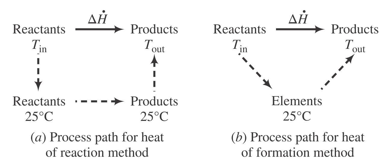
| Description | Equations |
|---|---|
| Enthalpy change of heat of reaction method | $\Delta \dot{H} = \sum\limits_{\text{rxn}} \xi \Delta H_{\text{rxn}}^\circ + \sum \dot{n}_{\text{out}}\hat{H}_{\text{out}} - \sum \dot{n}_{\text{in}}\hat{H}_{\text{in}}$ |
| Enthalpy change of heat of formation method | $\Delta \dot{H} = \sum \dot{n}_{\text{out}}\hat{H}_{\text{out}} - \sum \dot{n}_{\text{in}}\hat{H}_{\text{in}}$ |