CHEM E 435 Transport Process III

Separation Processes

Types of Separations

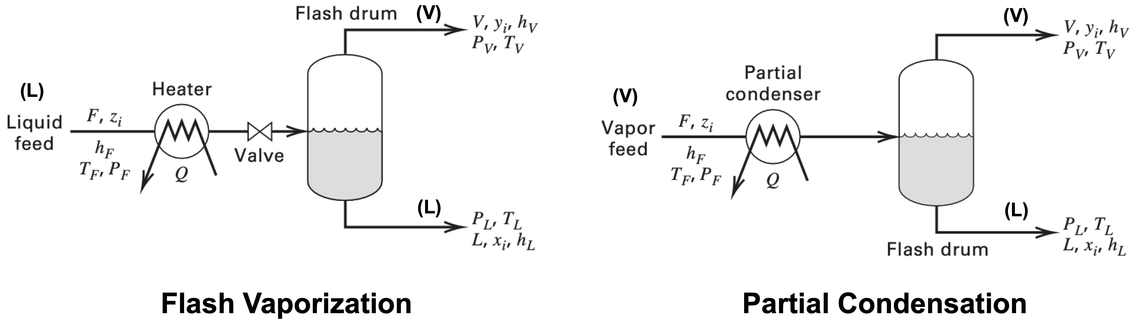
Separations by phase creation

Separation Operation	Feed Phase	Created Phase	Separating Agent
Partial condensation/vaporization	V and/or L	L or V	Heat transfer (ESA)
Flash vaporization	L	V	Pressure reduction
Distillation	V and/or L	V and L	Heat transfer (ESA) and sometimes shaft work (ESA)

Separations by phase addition

Separation Operation	Feed Phase	Created Phase	Separating Agent
Absorption	V	L	Liquid absorbent (MSA)
Stripping	L	V	Stripping vapor (MSA)
Liquid-liquid extraction	L	L	Liquid solvent (MSA)
Adsorption	V or L	S	Solid adsorbent (MSA)

Separations by barrier

Separation Operation	Feed Phase	Barrier	Separating Agent
Dialysis	L	Microporous membrane	Pressure (ESA)
Reverse osmosis	L	Microporous membrane	Pressure (ESA)
Gas permeation	Vapor	Nonporous membrane	Pressure (ESA)
Pervaporation	L	Nonporous membrane	Pressure and heat transfer (ESA)

Separations by external field/gradient

• Centrifugation - pressure gradient
• Thermal diffusion - temperature gradient
• Electrolysis
• Electrodialysis - permeable membrane with fixed charge
• Electrophoresis - electric field
• Magnetophoresis - magnetic field
• Crystallization - solubility

Thermodynamics Review

Description	Equations
Equilibrium conditions	$\begin{aligned}T_1 &= T_2 \\ P_1 &= P_2 \\ \bar{f}_2 &= \bar{f}_2 \\ a_1 &= a_2\end{aligned}$
Fugacity	$\bar{f}_i = \bar{f}_i^\circ \exp\left(\dfrac{\mu_i}{RT}\right)$
Fugacity coefficient	$\phi_i = \dfrac{f_i}{P}$
Partial fugacity coefficient	$\phi_i = \dfrac{f_i}{x_iP}$
Activity	$a_i = \dfrac{\bar{f}_i}{f_i^\circ}$
Activity coefficient	$\gamma_i = \dfrac{a_i}{x_i}$

$K$-values

Description	Equations
$K$-value (vapor-liquid equilibrium ratio)	$K_i = \dfrac{y_i}{x_i}$
Distribution ratio (partition coefficient, liquid-liquid equilibrium ratio	$K_{D_i} = \dfrac{x_i^\alpha}{x_i^\beta}$
Relative volatility	$\alpha_{i, j} = \dfrac{K_i}{K_j}$
Relative selectivity	$\beta{i, j} = \dfrac{K_{D_i}}{K_{D_j}}$
Raoult’s law ★ Ideal solution	$K_i = \dfrac{P_i^*}{P}$
Modified Raoult’s law ★ Low pressure	$K_i = \gamma_{i, L}\dfrac{P_i^*}{P}$
Poynting correction ★ Moderate pressure	$K_i = \gamma_{i, L}\phi_{i, V}^\mathrm{sat}\left(\dfrac{P_i^\mathrm{sat}}{P}\right) \exp\left[\dfrac{1}{RT}\displaystyle\int^P_{P_i^{\mathrm{sat}}} v_{i, L} dP \right]$
Henry’s law ★ Dilute species	$K_i = \dfrac{H_i}{P}$

Mass Transfer and Diffusion

Steady-state ordinary molecular diffusion (OMD)

Description	Equations
Fick’s first law Molecular diffusion flux of species A	$\begin{aligned} J_{A} &= -cD_{AB}\dfrac{dx_A}{dx} \\ &= -D_{AB} \dfrac{dc_A}{dz} \end{aligned} \newline j_{A} = -\rho D_{AB}\dfrac{dw_A}{dz}$
Bulk flow flux	$N = N_A + N_B$
Bulk flow flux of species A	$x_A N$
Molar flux of species A (definition)	$N_A = \dfrac{\dot{n}_A}{A}$
Molar flux of species A ★ No eddie diffusion flux	$\begin{aligned} N_A &= \text{bulk flow flux} + \text{molecular diffusion flux}\\ N_A &= x_A N - cD_{AB} \dfrac{dx_A}{dz} \end{aligned}$
Total velocity of species A	$v_A = \dfrac{N_A}{c_A}$
Molar-average mixture velocity	$v_M = v_Ax_A + v_Bx_B$
Diffusion velocity of species A	$v_{D, A} = \dfrac{J_A}{c_A}$
Velocity relations	$v_A = v_M + v_{D, A}$

Equimolar counter diffusion (EMD)

Description	Equations
Equimolar counter diffusion	$N_A = - N_B$
No bulk flow	$N = 0$
Molar flux of species A Molecular diffusion flux of species A	$N_A = J_A = -cD_{AB} \dfrac{\Delta x_A}{\Delta z}$
Concentration profile of species A	$c_A = c_{A0} - \dfrac{J_A z}{D_{AB}}$
Concentration profile of species B	$c_B = c_{B0} + \dfrac{J_A (z-L)}{D_{AB}}$

Unimolecular diffusion (UMD)

Description	Equations
Stagnant B	$N_B = 0$
Molar flux of species A Bulk flow flux	$N = N_A$
Molar flux of species A	$N_A = \dfrac{cD_{AB}}{z - z_1} \ln\left(\dfrac{1 - x_A}{1 - x_{A, 1}}\right)$
Molar flux of species A	$N_A = -\dfrac{cD_{AB}}{(1 - x_A)_{\mathrm{LM}}} \dfrac{\Delta x_A}{\Delta z}$
Dilute A reduces UMD to EMD (no bulk flow)	$(1 - x_A)_{\mathrm{LM}} \approx 1 \quad \text{if } x_A \to 0$
Log-mean	$x_{\mathrm{LM}} = \dfrac{x_2 - x_1}{\ln(x_2/x_1)}$
Composition profile	$x_A(z) = 1 - (1 - x_A) \exp\left[\dfrac{N_A (z - z_1)}{cD_{AB}}\right]$
Molecular diffusion and bulk flow flux of species	$J_A = x_B N = - J_B$
Changing liquid level of A with stagnant B	$N_A = -\dfrac{cD_{AB}}{(1 - x_A)_{\mathrm{LM}}} \dfrac{\Delta x_A}{z} = \dfrac{\rho_A}{\mathcal{M}_A}\dfrac{dz}{dt}$

Diffusivity

Diffusivity of gas mixtures

Description	Equations
Fuller-Schettler-Giddings correlation ★ Low pressure (0 - 10 atm) ★ $D_{AB} \ [\mathrm{cm^2/s}]$ ★ $P \ [\mathrm{atm}], T \ [\mathrm{K}]$ ★ $\mathcal{M}_{AB} \ [\mathrm{g/mol}]$	$D_{AB} = D_{BA} = \dfrac{0.00143 T^{1.75}}{P \mathcal{M}_{AB}^{1/2} \left[(\sum_V)_A^{1/3} + (\sum_V)_B^{1/3}\right]^2} \newline $
Effective molecular mass	$\mathcal{M}_{AB} = \dfrac{2}{\dfrac{1}{\mathcal{M}_A} + \dfrac{1}{\mathcal{M}_B}}$
Summation of atomic and structural diffusion volumes (Table 3.1)	$\sum_V$
Takahashi correlation ★ High pressure (Figure 3.3)	$\dfrac{D_{AB} P}{(D_{AB}P)_{\text{low }P}} = \mathrm{const}$
Molar averaged reduced properties	$T_r = x_A T_{r, A} + x_B T_{r, B} \newline P_r = x_A P_{r, A} + x_B P_{r, B}$

Diffusivity of nonelectrolyte liquid mixtures

Description	Equations
Stoke-Einstein equation ★ Infinite dilution	$(D_{AB})_\infty = \dfrac{RT}{6\pi \mu_B R_A N_A} \propto \dfrac{T}{\mu_B R_A}$
Wilke-Chang equation ★ Low pressure (0 - 10 atm) ★ $D_{AB} \ [\mathrm{cm^2/s}]$ ★ $\mu_B \ [\mathrm{cP}], T \ [\mathrm{K}]$ ★ $\mathcal{M}_{AB} \ [\mathrm{g/mol}]$ ★ $v_A \ [\mathrm{cm^3/mol}]$	$(D_{AB})_\infty = 7.4\times 10^{-8} \dfrac{(\phi_B \mathcal{M}_B)^{1/2}T}{\mu_B v_A^{0.6}}$
Hayduk-Minhas correlation (Modified Wilke-Chang equation)	$(D_{AB})_\infty = 13/3\times 10^{-8} \dfrac{T^{1.47}\mu_B^\varepsilon}{v_A^{0.71}} \newline \varepsilon = \dfrac{10.2}{v_A} - 0.791$

Film theory for mass transfer at fluid-fluid interface

Single film theory

Description	Equations
Concentration and mole fraction	$c_A = x_Ac$
Mass transfer coefficient (no bulk flow)	$k_c = \dfrac{D_{AB}}{\delta}$
Mass transfer coefficient (with bulk flow)	$k'_c = \dfrac{D_{AB}}{\delta (1 - x_A)_{\mathrm{LM}}}$
Molar flux of species A ★ Interface (i), bulk (b)	$N_A = \pm k_c (c_{A, i} - c_{A, b}) \newline N_A = \pm k'_c (c_{A, i} - c_{A, b})$
Film thickness	$\delta = \dfrac{D_{AB}}{k_c} = \dfrac{D_{AB}}{k'_c (1 - x_A)_{\mathrm{LM}}}$

Mass transfer coefficient and driving force

Driving Force	Mass Transfer Coefficient	Equations
Concentration (liquid)	$k_c \ [\mathrm{m/s}]$	$N_A = \pm k_c (c_{A, i} - c_{A, b})$
Pressure (vapor)	$k_p \ [\mathrm{mol/m^2 \cdot s \cdot Pa}]$	$N_A = \pm k_p (P_{A, i} - P_{A, b})$
Mole fraction (liquid)	$k_x \ [\mathrm{mol/m^2 \cdot s}]$	$N_A = \pm k_x (x_{A, i} - x_{A, b})$
Mole fraction (vapor)	$k_y \ [\mathrm{mol/m^2 \cdot s}]$	$N_A = \pm k_y (y_{A, i} - y_{A, b})$

Description	Equations
Liquid phase coefficient conversion	$k_x = k_c c = k_c \dfrac{\rho_L}{\mathcal{M}_L}$
Vapor phase coefficient conversion	$k_y = k_p P = (k_c)_g c = (k_c)_g \dfrac{P}{RT} = (k_c)_g \dfrac{\rho_G}{\mathcal{M}_G}$
Liquid phase bulk flow correction	$k' = \dfrac{k}{(1 - x_A)_{\mathrm{LM}}}$
Gas phase bulk flow correction	$k' = \dfrac{k}{(1 - y_A)_{\mathrm{LM}}}$

Two-film theory

Based on	Overall Mass Transfer Coefficient	Equations	Fictitious properties
Liquid phase	$\dfrac{1}{K_L} = \dfrac{H_A}{k_p} + \dfrac{1}{k_c}$	$N_A = \pm K_L (c_A^* - c_{A, b})$	$c_A^* = P_{A, b} H_A$
Gas phase	$\dfrac{1}{K_G} = \dfrac{1}{k_p} + \dfrac{1}{H_A k_c}$	$N_A = \pm K_G (P_{A, b} - P_A^*)$	$P_A^* = \dfrac{c_{A, b}}{H_A}$
Liquid phase mole fraction	$\dfrac{1}{K_x} = \dfrac{1}{K_a k_y} + \dfrac{1}{k_x}$	$N_A = \pm K_y (y_{A, b} - y_{A}^*)$	$y_A^* = x_{A, b}K_A$
Gas phase mole fraction	$\dfrac{1}{K_y} = \dfrac{1}{k_y} + \dfrac{K_A}{k_x}$	$N_A = \pm K_x (x_{A}^* - x_{A, b})$	$x_A^* = \dfrac{y_{A, b}}{K_A}$

Single Equilibrium Stages

Degrees of freedom

Description	Equations
Gibbs' phase rule	$\mathrm{DOF = component - phase + 2}$
Degree of freedom	$\small\text{DOF = \# intensive variables} - \text{\# independent eqns}$
Azeotrope	$x_i = y_i$
$q$-line	$y_H = \left[\dfrac{(V/F) - 1}{(V/F)}\right] x_H + \left[\dfrac{1}{(V/F)}\right] z_H$

Rachford-Rice algorithm for isothermal flash calculation

Description	Equations
Road map	Known - $K_i, z_i, F$ Solve - $\Psi \to V \to L \to x_i, y_i \to Q$
Vapor-to feed ratio	$\Psi \equiv \dfrac{V}{F}$
Objective function ★ Derived from $\sum y_i - \sum x_i = 0$	$f(\Psi) = \displaystyle\sum_i \dfrac{z_i (1 - K_i)}{[1 + \Psi(K_i - 1)]} = 0$
Derivative of objective function	$f'(\Psi) = \displaystyle\sum_i \dfrac{z_i (1 - K_i)^2}{[1 + \Psi(K_i - 1)]^2}$
Newton’s method for root finding	$\Psi_{n+1} = \Psi_n - \dfrac{f(\Psi_n)}{f'(\Psi_n)}$
Vapor molar flow rate	$V = \Psi F$
Liquid molar flow rate	$L = F - V$
Vapor mole fraction	$x_i = \dfrac{z_i}{1 + \Psi(K_i - 1)}$
Liquid mole fraction	$y_i = \dfrac{z_i K_i}{1 + \Psi(K_i - 1)}$
Heat	$Q = h_V V + h_L L - h_F F$

Bubble and dew point calculations

Description	Equations
Bubble point	$\Psi = 0 \newline \sum z_i K_i = 1 \newline \sum \dfrac{y_i}{P_i^* (T)} = \dfrac{1}{P}$
Dew point	$\Psi = 1 \newline \sum \dfrac{z_i}{K_i} = 1 \newline \sum x_i P_i^* (T) = P$

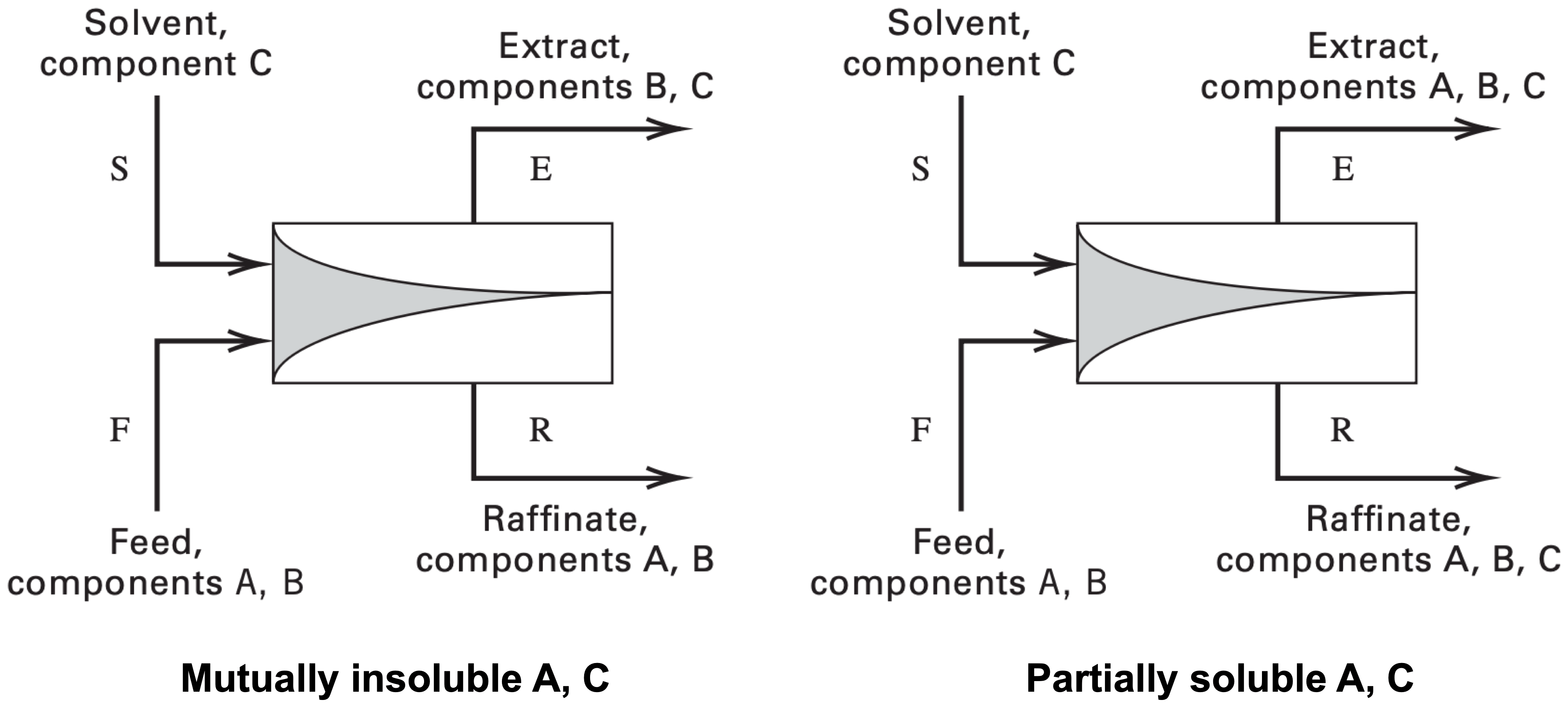
Ternary liquid-liquid extraction

Description	Equations
Mass fraction	$x_i = \dfrac{m_i}{m}$
Mass ratio	$X_i = \dfrac{m_i}{m - m_i}$
Conversion between mass fraction and ratio	$X_i = \dfrac{x_i}{1 - x_i} \newline x_i = \dfrac{X_i}{1 - X_i}$
Solute balance ★ Solvent A, Solute B ★ Feed F, Solvent S, Extract E, Raffinate R	$\begin{aligned} F_B &= E_B + R_B & \\ X_{F, B} F_A &= Y_{E, B} S + X_{R, B}F_A & Y_{E, B} = K'_{D_B} X_{R, B} \\ X_{F, B}F_A &= K'_{D_B} X_{R, B}S + X_{R, B}F_A & \\ X_{R, B} &= \dfrac{X_{F, B} F_A}{F_A + K'_{D_B} S} \end{aligned}$
Extraction factor of solute B	$\mathcal{E} = \dfrac{K'_{D_B} S}{F_A}$
Fraction of solute B unextracted	$\dfrac{X_{R, B}}{X_{F, B}} = \dfrac{1}{1 + \mathcal{E}}$

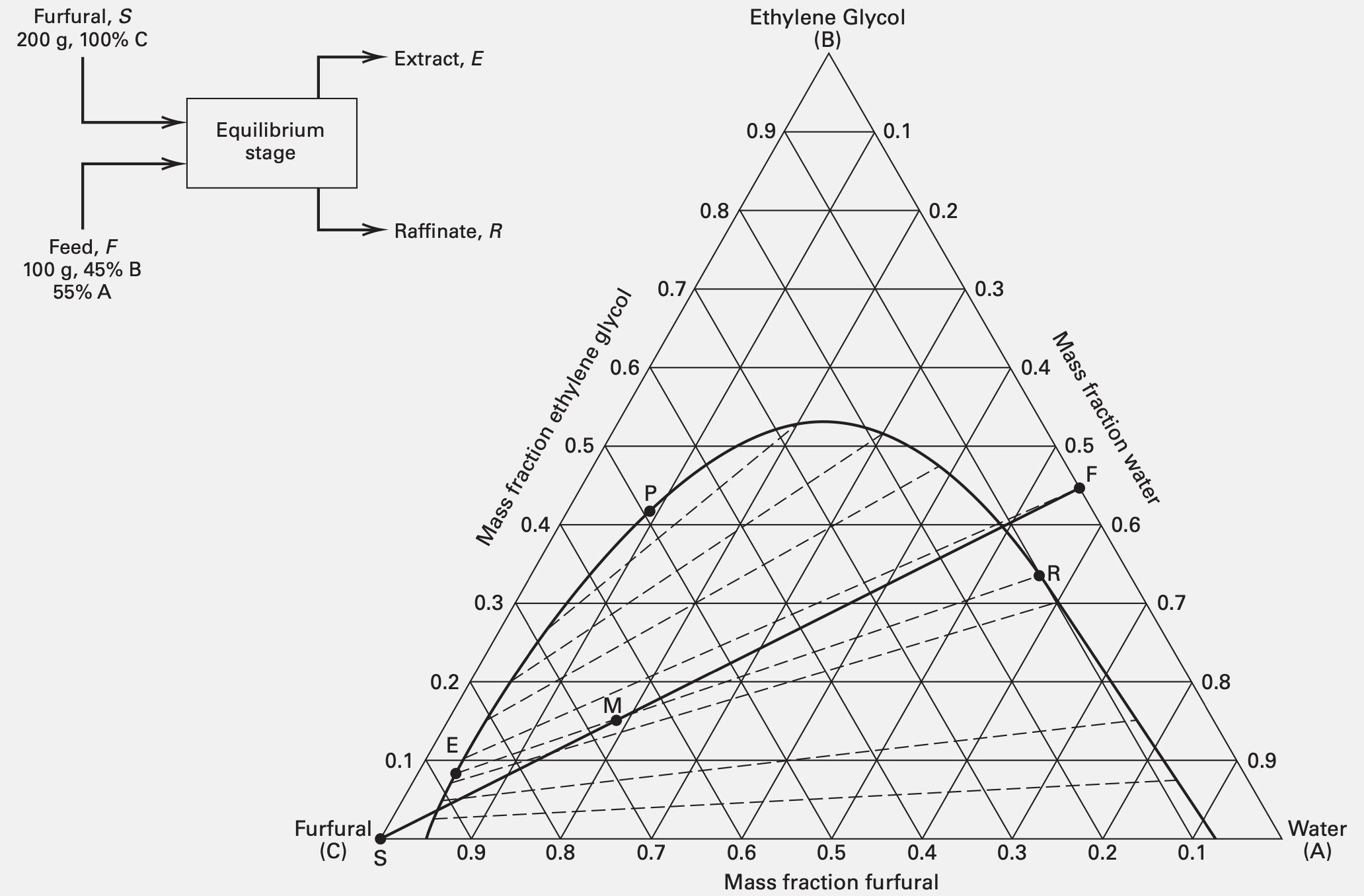
Ternary phase diagram

General principles are the same for different types of ternary phase diagrams. Here, algorithm for using equilateral ternary phase diagrams is presented.

• Identify chemical species at the apexes: feed solvent (A), feed solute (B), and pure solvent (S)
  • Apexes are pure components
  • Lines parallel to the apex are used to read values
  • Label each side of the triangle according to the apex
• Identify compositions of entering streams: feed (F) and solvent (S)
  • Assume feed only contains A and B, and solvent is pure S
  • Calculate composition of mixture (M) with component balances
    • $x_{M, A} = \dfrac{x_{F, A} F}{F + S}, \quad x_{M, B} = \dfrac{x_{F, B} F}{F + S}, \quad x_{M, C} = \dfrac{S}{F + S}$
• Interpolate tie line on the ternary phase diagram
• Identify compositions of exiting streams: extract (E) and raffinate (R)
  • E and R lies on the intersection of tie line and miscibility boundary (binodal) curve
  • E has a larger S component than R (extracted component is dissolved in solvent), being closer to point S
• Identify plait point (P)
  • P lies between E and R on the miscibility boundary curve
  • P the the point where E and R merge together and tie line collapses to a point
• Determine flow rate ratio with inverse level rule
  • $\dfrac{E}{F + S} = \dfrac{E}{E + R} = \dfrac{\overline{MR}}{\overline{ER}}, \quad \dfrac{E}{R} = \dfrac{\overline{MR}}{\overline{ME}}$

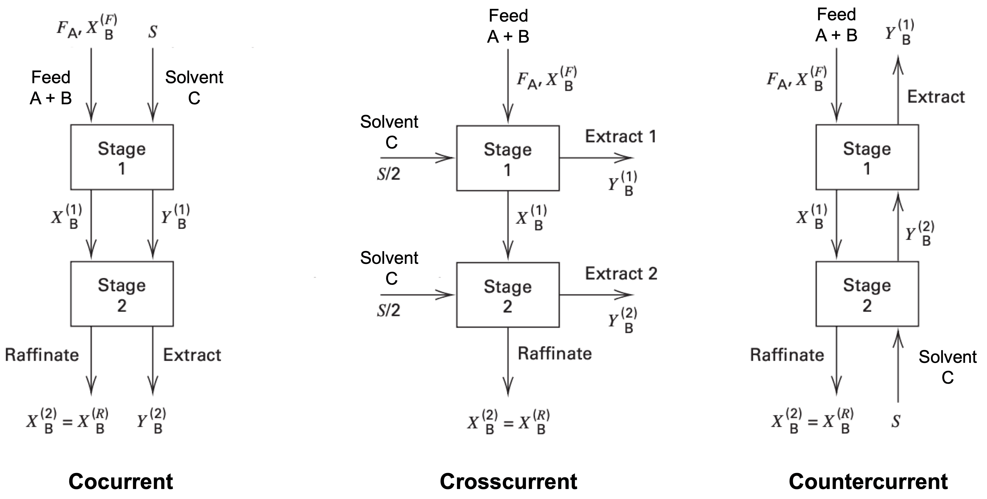
Multistage Cascades

Configuration	Fraction of solute B unextracted
Single stage	$\dfrac{X_{R, B}}{X_{F, B}} = \dfrac{1}{1 + \mathcal{E}}$
Cocurrent cascade ($N$ stages)	$\dfrac{X_{N, B}}{X_{F, B}} = \dfrac{1}{1 + \mathcal{E}}$
Crosscurrent cascade ($N$ stages)	$\dfrac{X_{N, B}}{X_{F, B}} = \dfrac{1}{(1 + \mathcal{E}/N)^N}$
Crosscurrent cascade ($\infty$ stages)	$\dfrac{X_{\infty, B}}{X_{F, B}} = \dfrac{1}{\exp(\mathcal{E})}$
Countercurrent cascade ($N$ stages)	$\dfrac{X_{R, B}}{X_{F, B}} = \left[\displaystyle\sum_{n = 0}^N \mathcal{E}^n\right]^{-1} = \dfrac{\mathcal{E} - 1}{\mathcal{E}^{N+1} - 1}$
Countercurrent cascade ($\infty$ stages)	$\begin{cases} \dfrac{X_{\infty, B}}{X_{F, B}} = 0, & \mathcal{E} \in [1, \infty) \\ \dfrac{X_{\infty, B}}{X_{F, B}} = 1 - \mathcal{E}, & \mathcal{E} \in (-\infty, 1) \end{cases}$

Absorption and Stripping

Graphical method for trayed towers

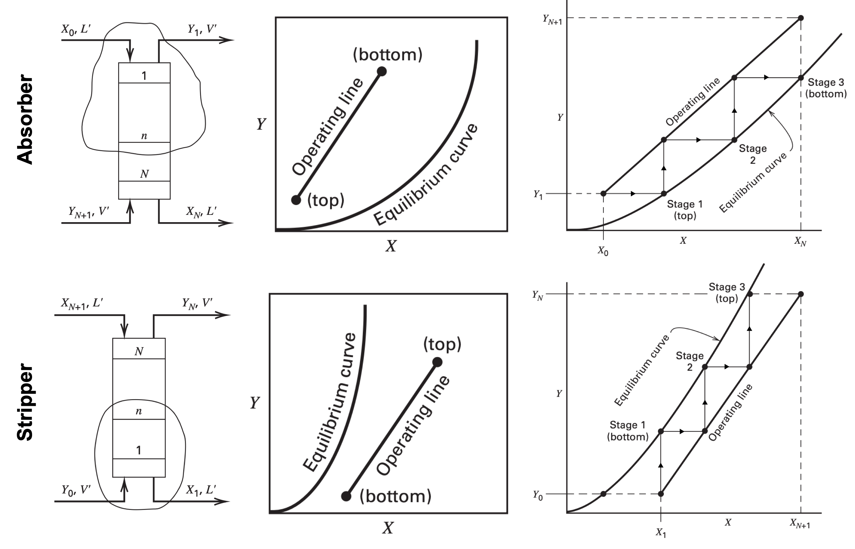
• Construct the equilibrium curve from thermodynamics
  • $K_n = \dfrac{y_n}{x_n} = \dfrac{Y_n}{X_n}\dfrac{1 + X_n}{1 + Y_n} \implies Y_n = \dfrac{K_n X_n}{1 + X_n - K_n X_n}$
• Identify absorption and stripping process
  • Absorption - Use liquid to remove components from gas mixture
  • Stripping - Use gas to remove components from liquid mixture
• Construct operating line for $\infty$ stages for $L'_{\min}$ or $V'_{\min}$
  • Absorption ($L'_{\min}$)
    • Identify (liquid in, gas out) = $(X_0, Y_1)$
    • Identify (liquid out, gas in) = $(X_N, Y_{N+1})$ with minimum operating line intersects and ends at the equilibrium curve
  • Stripping ($V'_{\min}$)
    • Identify (gas in, liquid out) = $(X_1, Y_0)$
    • Identify (liquid out, gas in) = $(X_{N+1}, Y_N)$ with minimum operating line intersects and ends at the equilibrium curve
  • Slope of operating line = $\dfrac{L'}{V'}$
• Determine number of equilibrium stages for $L'$ and $V'$
  • Absorption ($L'$)
    • Construct operating line with point (liquid in, gas out) = $(X_0, Y_1)$ and slope = $\dfrac{L'}{V'}$
    • From $(X_0, Y_1)$, draw horizontal line toward the equilibrium curve and vertical lines back to the operating line until it reaches $(X_N, Y_{N+1})$
  • Stripping ($V'$)
    • Construct operating line with point (gas in, liquid out) = $(X_1, Y_0)$ and slope = $\dfrac{L'}{V'}$
    • From $(X_1, Y_0)$, draw horizontal line toward the equilibrium curve and vertical lines back to the operating line until it reaches $(X_{N+1}, Y_N)$
  • The number of equilibrium stages is the number of intersections on the equilibrium curve
    • Interpolate number of stages if not exact

Absorption

Description	Equations
Absorption operating line	$Y_{n+1} = X_n \dfrac{L'}{V'} + Y_1 - X_0 \dfrac{L'}{V'}$
Absorbent flow rate	$L' = V' \dfrac{Y_{N+1} - Y_1}{X_N - X_0}$
Minimum absorbent flow rate ($\infty$ stages)	$L'_{\min} = V' K_N \cdot (\text{fraction solute absorbed})$
Absorption factor	$\mathcal{A} = \dfrac{L}{K V}$

Stripping

Description	Equations
Stripping operating line	$Y_{n} = X_n \dfrac{L'}{V'} + Y_0 - X_1 \dfrac{L'}{V'}$
Stripping agent flow rate	$V' = L'\dfrac{X_{N} - X_1}{Y_N - Y_0}$
Minimum stripping agent flow rate ($\infty$ stages)	$V'_{\min} = \dfrac{L'}{K_N} \cdot (\text{fraction solute stripped})$
Stripping factor	$\mathcal{S} = \dfrac{V}{L}K$
Relating stripping factor and adsorption factor	$\mathcal{S} = \dfrac{1}{\mathcal{A}}$

Stage efficiency and packed columns

Description	Equations
Overall stage efficiency	$E_o = \dfrac{\text{\# theoretical stages}}{\text{\# actual stages}}$
Drickamer and Bradford correlation ★ Hydrocarbons, $\mu_L \in (0.2, 1.6) \ \mathrm{cP}$	$E_o [\%] = 19.2 - 57.8 \log(\mu_L)$
Height equivalent to a theoretical plate (HETP)	$\mathrm{HETP} = \dfrac{l_T}{N_t} = \dfrac{\text{packed height}}{\text{\# equiv eqm stages}}$
Packed height	$l_T = H_{OG}N_{OG}$
Overall height of a transfer unit (HTU)	$H_{OG} = \dfrac{V}{K_y a A_c}$
Overall number of transfer unit (NTU)	$N_{OG} = \displaystyle\int_{y_{\text{out}}}^{y_{\text{in}}}\dfrac{dy}{y - y^*}$
Overall volumetric mass transfer coefficient	$K_y a$

Distillation of Binary Mixtures

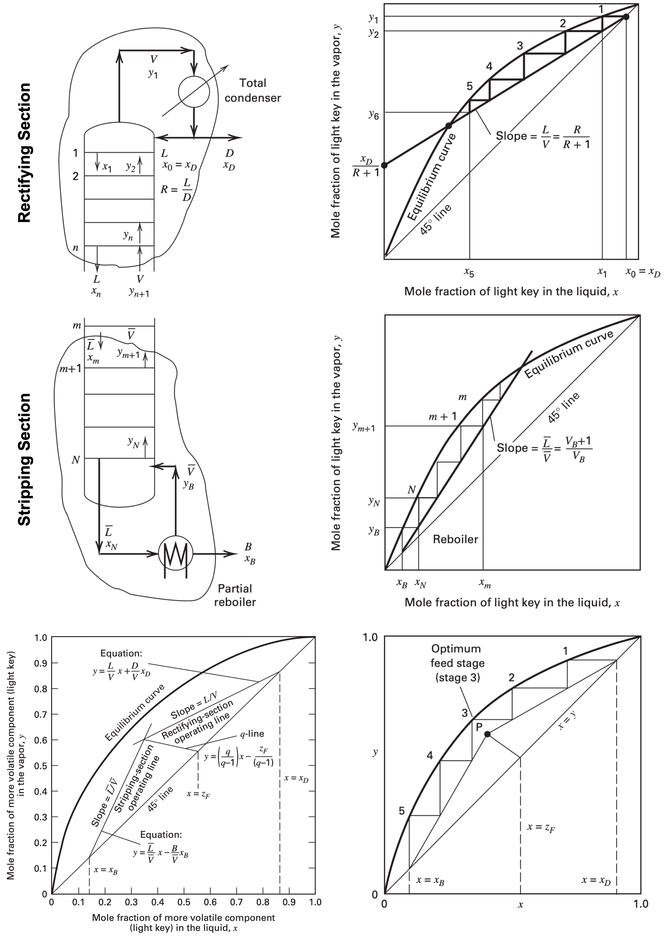
McCabe-Thiele graphical method for trayed towers

Description	Equations
McCabe-Thiele assumptions	1. Equal and constant $\Delta H_{\text{vap}}$ 2. Negligible $C_P \Delta T$ and $\Delta H_{\text{mix}}$ 3. Insulated column $q = 0$ 4. No pressure drop $\Delta P = 0$
Constant molar overflow in rectifying section	$L_1 = L_i = L \newline V_1 = V_i = V$
Constant molar overflow in stripping section	$\overline{L}_1 = \overline{L}_i = \overline{L} \newline \overline{V}_1 = \overline{V}_i = \overline{V}$
Non-equal flow rate in rectifying and stripping sections	$L \not= \overline{L} \newline V \not= \overline{V}$
Reflux ratio	$R = \dfrac{L}{D}$
Boilup ratio	$V_B = \dfrac{\overline{V}}{B}$
Equilibrium curve	$y_1 = \dfrac{\alpha_{1, 2}x_1}{1 + x_1(\alpha_{1, 2} - 1)}$
Rectifying section operating line	$y = \left(\dfrac{R}{R + 1}\right)x + \left(\dfrac{x_D}{R + 1}\right)$
Stripping section operating line	$y = \left(\dfrac{V_B + 1}{V_B}\right)x - \left(\dfrac{x_B}{V_B}\right)$
$q$-parameter	$\begin{cases} q > 1 & \text{subcooled liq} \\ q = 1 & \text{saturated liq (bubble pt)} \\ q \in (0, 1) & \text{liq + vap} \\ q = 0 & \text{saturated vap (dew pt)} \\ q < 0 & \text{superheated vap} \end{cases}$
$q$-parameter	$q = \dfrac{\overline{L} - L}{F} = 1 + \dfrac{\overline{V} - V}{F}$
$q$-line	$y = \left(\dfrac{q}{q - 1}\right)x + \left(\dfrac{z_F}{q - 1}\right)$

Limiting conditions

Description	Equations
Total reflux (Useless)	$R_\infty = \infty \newline N_{\min} = 0 \newline L = V \newline D = B = 0$
Minimum reflux	$R_{\min} = \dfrac{(L/V)_{\min}}{1 - (L/V)_{\min}} \newline N_\infty = \infty \newline V_{B, \min} = \dfrac{1}{(\overline{L}/\overline{V})_{\min} - 1}$
Perfect separation	$x_D = 1, \quad x_B = 0 \newline R \ge R_{\min} \begin{cases} R_{\min} = \dfrac{1}{z_F (\alpha_{1, 2} - 1)} & q = 1 \\ R_{\min} = \dfrac{\alpha_{1, 2}}{z_F (\alpha_{1, 2} - 1)} - 1 & q = 0 \end{cases}$

Membrane Separations

Description	Equations
Transmembrane molar flux	$\begin{aligned}N_i &= \dfrac{P_{M, i}}{l_M} \cdot (\text{driving force}) \\ &= \bar{P}_{M, i} \cdot (\text{driving force}) \end{aligned}$
Permeance	$\bar{P}_{M, i} = \dfrac{P_{M, i}}{l_M}$
Permeability	$P_{M, i} = \bar{P}_{M, i} l_M$
Selectivity	$S_{i, j} = \dfrac{P_{M, i}}{P_{M, j}}$
Gas permeability unit	$\begin{aligned}&1 \ \mathrm{barrer} \\ &= 10^{-10} \ \mathrm{cm^3_{STP} \cdot cm/(cm^2 \cdot s \cdot cmHg)} \\ &= 3.35 \times 10^{-16} \ \mathrm{mol \cdot m / (m^2 \cdot s \cdot Pa)} \\ &= 5.58 \times 10^{-12} \ \mathrm{lbmol \cdot ft / (ft^2 \cdot h \cdot psi)}\end{aligned}$
Mole of gas in standard temperature and pressure (STP)	$1 \ \mathrm{mol} \sim 22.4 \ \mathrm{L_{STP}}$

Transport through porous membranes

Bulk flow

Description	Equations
Hagen-Poiseuille flow ★ Laminar flow $\mathrm{Re} < 2100$	$v = \dfrac{D^2}{32\mu L}(P_0 - P_L)$
Pore number density	$n = \dfrac{n_\text{total}}{A_c} = \dfrac{\text{total \# of pores}}{\text{membrane cross sectional area}}$
Porosity (void fraction) ★ Straight cylindrical pore	$\varepsilon = \frac{1}{4}n\pi D^2$
Bulk flow flux ★ Straight cylindrical pore	$\begin{aligned}N &= v\rho\varepsilon \\ &= \dfrac{\varepsilon\rho D^2}{32 \mu l_M} (P_0 - P_L) \\ &= \dfrac{n\pi\rho D^4}{128 v l_M}(P_0 - P_L)\end{aligned}$
Empirical hydraulic diameter	$d_H = \dfrac{4\varepsilon}{a_v}$
Specific surface area	$a_v = \dfrac{a}{1 - \varepsilon}$
Total pore surface area	$a = a_v (1 - \varepsilon)$
Tortuosity correction of membrane width	$\tau l_M$
Bulk flow flux ★ General pore	$N = \dfrac{\rho\varepsilon^2}{2(1-\varepsilon)^2 \tau a_v^2 \mu l_M}(P_0 - P_L)$
Ergun equation	$\dfrac{P_0 - P_L}{l_M} = \dfrac{150 \mu v_0 (1-\varepsilon)^2}{D_P^2 \varepsilon^3} + \dfrac{1.75 \rho v_0^2 (1 - \varepsilon)}{D_P \varepsilon^3}$
Mean spherical particle diameter	$D_P = \dfrac{6}{a_v}$

Liquid diffusion

Description	Equations
Concentration driving force	$\Delta c \not= 0 \newline \Delta P = 0$
Transmembrane mass flux	$N_i = \dfrac{D_{e, i}}{l_M}(c_{i, 0} - c_{i, L})$
Effective diffusivity	$D_{e, i} = \dfrac{\varepsilon D_i}{\tau} K_{r, i}$
Restrictive factor of solute	$K_r = \left[ 1 - \dfrac{d_m}{d_p}\right]^4$
Selectivity	$S_{i, j} = \dfrac{D_i K_{r, i}}{D_j K_{r, j}}$

Gas diffusion

Description	Equations
Transmembrane molar flux ★ Ideal gas, uniform transmembrane T, P	$\begin{aligned} N_i &= \dfrac{c_M}{P}\dfrac{D_{e, i}}{l_M}(P_{i, 0} - P_{i, L}) \\ &= \dfrac{1}{RT}\dfrac{D_{e, i}}{l_M}(P_{i, 0} - P_{i, L}) \end{aligned}$
Effective diffusivity	$D_{e, i} = \dfrac{\varepsilon}{\tau} \left[\dfrac{1}{(1/D_i) + (1/D_{K, i})}\right]$
Knudsen diffusivity of straight cylindrical pore ★ Kinetic theory of gas	$D_{K, i} \ [\mathrm{cm/s}] = 4850 d_p \ [\mathrm{cm}] \sqrt{\dfrac{T}{\mathcal{M}_i}\dfrac{[\mathrm{K}]}{[\mathrm{g/mol}]}}$
Selectivity of Knudsen diffusion ★ $D_i \gg D_{K, i}$ ★ $D_{e, i} \sim D_{K, i}$	$S_{i, j} = \dfrac{P_{M, i}}{P_{M, j}} = \sqrt{\dfrac{\mathcal{M}_j}{\mathcal{M}_i}}$

Transport through nonporous (dense) membranes

Solution-diffusion of liquid mixtures

Description	Equations
Thermodynamic equilibrium partition coefficient	$K_i = \dfrac{c_i}{c_i'}$
Transmembrance mass flux ★ Fick’s law	$N_i = \dfrac{D_i}{l_M}(c_{i, 0} - c_{i, L})$
Transmembrance mass flux ★ $K_{i, 0} = K_{i, L} = K_{i}$	$N_i = \dfrac{K_i D_i}{l_M}(c'_{i, 0} - c'_{i, L})$
Transmembrance mass flux ★ No mass transfer resistance in fluid boundary layers ★ $c'_{i, 0} = c_{i, F}$ and $c'_{i, L} = c_{i, P}$	$N_i = \dfrac{K_i D_i}{l_M}(c_{i, F} - c_{i, P})$

Solution-diffusion of gas mixtures

Description	Equations
Henry’s constant	$H_i = \dfrac{c_i}{P_i}$
Transmembrance mass flux ★ Fick’s law	$N_i = \dfrac{D_i}{l_M}(c_{i, 0} - c_{i, L})$
Transmembrance mass flux ★ $H_{i, 0} = H_{i, L} = H_{i}$	$N_i = \dfrac{H_i D_i}{l_M}(P_{i, 0} - P_{i, L})$
Transmembrance mass flux ★ No mass transfer resistance in external boundary layers ★ $P_{i, 0} = P_{i, F}$ and $P_{i, L} = P_{i, P}$	$N_i = \dfrac{H_i D_i}{l_M}(P_{i, F} - P_{i, P})$

Separation factor

Description	Equations
Ideal separation factor ★ Downstream permeate pressure negligible compared to upstream feed pressure ★ $x_{i, P} P_P \ll x_{i, F} P_F$ and $x_{j, P} P_P \ll x_{j, F} P_F$	$\alpha^*_{i, j} = \dfrac{H_i D_i}{H_j D_j} = \dfrac{P_{M, i}}{P_{M, j}}$
Separation factor	$\alpha_{i, j} = \alpha^*_{i, j} \left[\dfrac{(x_{j, F} / x_{j, P}) - r\alpha_{i, j}}{(x_{j, F} / x_{j, P}) - r}\right]$
Cut (fraction of feed permeated)	$\theta = \dfrac{\dot{n}_P}{\dot{n}_F}$

Summary of transport through membranes

Type of transport	Permselective	Membrane Type	Driving Force	Permeability
(L) Bulk flow	No	Macroporous	$\Delta P$	$\begin{aligned}P_M = \dfrac{\rho\varepsilon^3}{2(1 - \varepsilon)^2 \tau a_v^2 \mu}\end{aligned}$
(L) Molecular diffusion	Yes	Microporous	$\Delta c$	$P_M = D_{e, i} = \dfrac{\varepsilon D_i K_{r, i}}{\tau}$
(G) Molecular diffusion ★ high P ★ $d_p > d_m$	Yes	Microporous	$\Delta P_i \newline \Delta P = 0$	$P_{M, i} = \dfrac{D_{e, i}}{RT}$
(G) Knudsen diffusion ★ low P ★ $d_p \sim d_m$	Yes	Microporous	$\Delta P_i \newline \Delta P = 0$	$P_{M, i} = \dfrac{D_{e, i}}{RT}$
(L) Solution diffusion	Yes	Nonporous (dense)	$\Delta c$	$P_{M, i} = K_i D_i$
(G) Solution diffusion	Yes	Nonporous (dense)	$\Delta P_i \newline \Delta P = 0$	$P_{M, i} = H_i D_i$

Reverse osmosis

Description	Equations
Osmotic pressure ★ Equilibrium	$\Pi \equiv P_1 - P_{\ce{H2O}}$
Osmotic pressure of water	$\Pi_{\ce{H2O}} = 0$
Osmotic process	$P_1 - P_{\ce{H2O}} < \Pi$
Reverse osmotic process	$P_1 - P_{\ce{H2O}} > \Pi$
Osmotic pressure’s thermodynamic derivation ★ Between pure water and solution ★ Solvent $A$, solute $B$	$\Pi = -\dfrac{RT}{v_{A}} \ln(x_A \gamma_A)$
Osmotic pressure ★ Ideal solution, dilute $B$	$\Pi = \dfrac{RT n_B}{v_A} = \dfrac{RTc_B}{\mathcal{M}_B}$

Seawater reverse osmosis

Description	Equations
Seawater as solution 1; salt as solute B	$\ce{A} = \text{water} = \ce{H2O} \newline \ce{B} = \text{salt} = \ce{S}$
Molar mass	$\mathcal{M} = \dfrac{m}{n}$
Molarity (molar concentration)	$M = \dfrac{n}{V} = \dfrac{\mathrm{wt \% \ S}}{100 \% - \mathrm{wt \% \ S}}\dfrac{\rho_{\ce{H2O}}}{\mathcal{M}_S}$
Seawater osmotic pressure correlation	$\Pi \ [\mathrm{psia}] = 1.12 T \ [\mathrm{K}] \sum M_i \ [\mathrm{mol/L}]$
Transmembrane molar flux of water (solvent A)	$N_{\ce{H2O}} = \dfrac{P_{M, \ce{H2O}}}{l_M} (\Delta P - \Delta \pi)$
Salt passage	$\mathrm{SP} = \dfrac{c_{S, P}}{c_{S, F}}$
Salt rejection	$\mathrm{SR} = 1 - \mathrm{SP}$
Concentration polarization factor	$\Gamma \equiv \dfrac{c_{S, i} - c_{S, F}}{c_{S, F}} = \dfrac{N_{\ce{H2O}} (\mathrm{SR})}{k_S}$
Significant concentration polarization	$\Gamma > 0.2$