CHEM E 326 Chemical Engineering Thermodynamics

Thermodynamic Properties and Data

Description	Equations
Mechanical equilibrium	$P_{\text{sys}} = P_{\text{surr}}$
Thermal equilibrium	$T_{\text{sys}} = T_{\text{surr}}$
Chemical equilibrium	$\mu(t_1) = \mu(t_2)$
Gibbs phase rule	$\mathcal{F} = 2 + c - p - r$
Quality	$x = \dfrac{n_v}{n_l + n_v} = \dfrac{v - v_l}{v_v - v_l}$
Critical point	$\left( \dfrac{\partial P}{\partial v} \right)_{T_c} = 0, \left( \dfrac{\partial^2 P}{\partial v^2} \right)_{T_c} = 0$

First Law of Thermodynamics

System Type	Equations
Closed systems	$\Delta u + \Delta e_K + \Delta e_P = q + w$
Closed systems	$\Delta u = q + w$
Open systems	$\dfrac{dU}{dt} = \sum\limits_{\text{in}}\dot{n}_i h_i + \sum\limits_{\text{out}}\dot{n}_i h_i + \dot{Q} + \dot{W}_s$
Open system at steady state	$0 = \sum\limits_{\text{in}}\dot{n}_i h_i + \sum\limits_{\text{out}}\dot{n}_i h_i + \dot{Q} + \dot{W}_s$

Description	Equations
Work	$w = - \int P_{\text{ext}} dv$
Enthalpy	$h = u + Pv$
Efficiency of irreversible isothermal expansion	$\eta = \dfrac{w_{\text{irrev}}}{w_{\text{rev}}}$
Efficiency of irreversible isothermal compression	$\eta = \dfrac{w_{\text{rev}}}{w_{\text{irrev}}}$

Heat capacity

Description	Equations
Constant volume heat capacity	$c_v = \left(\dfrac{\partial u}{\partial T}\right)_v$
Constant pressure heat capacity	$c_P = \left(\dfrac{\partial h}{\partial T}\right)_P$
Ideal gas heat capacity	$c_P = c_v + R$
Condensed phase heat capacity (l, s)	$c_P \approx c_v$
Mean heat capacity of gas	$\bar{c}_P = \dfrac{1}{T_2 - T_1} \displaystyle\int_{T_1}^{T_2} c_P(T) dT$

Enthalpy

Description	Equations
Enthalpy of vaporization	$\Delta h_{\text{vap}} = h_v - h_l$
Enthalpy of fusion	$\Delta h_{\text{fus}} = h_s - h_l$
Enthalpy of sublimation	$\Delta h_{\text{sub}} = h_v - h_s$
Enthalpy of phase change at any $T$	$\Delta h_{\text{vap}}(T) = \Delta h_{\text{vap}}(T_b) + \int_{T_b}^{T} (c_P^{v} - c_P^l)dT$
Enthalpy of reaction	$\Delta h_{\text{rxn}}^\circ = \sum \nu_i \Delta h_{f, i}$

Second Law of Thermodynamics

System Type	Equations
Isolated system	$\Delta S_{\text{univ}} \ge 0$
Closed system	$\Delta S_{\text{sys}} - \dfrac{Q_{\text{sys}}}{T_{\text{surr}}} \ge 0$
Open system	$\sum\limits_{\text{out}} \dot{n}_i s_i - \sum\limits_{\text{in}} \dot{n}_i s_i - \dfrac{\dot{Q}}{T_{\text{surr}}} + \dfrac{dS}{dt} \ge 0$
Open system at steady state	$\sum\limits_{\text{out}} \dot{n}_i s_i - \sum\limits_{\text{in}} \dot{n}_i s_i - \dfrac{\dot{Q}}{T_{\text{surr}}} \ge 0$

Description	Equations
Entropy	$ds = \dfrac{\delta q_{\text{rev}}}{T}$

Closed System Balance

Polytropic processes

Description	$\gamma$	Equation
Polytropic	-	$PV^\gamma = \text{const}$
Isobaric	$0$	$P = \text{const}$
Isothermal	$1$	$PV = \text{const}$
Isentropic	$k = \dfrac{c_P}{c_v}$	$PV^k = \text{const}$
Isochoric	$\infty$	$V = \text{const}$

Isothermal/Isoenergetic process

Isoenergetic process ($\Delta u = 0 \implies \Delta T = 0$) of ideal gas has similar analysis.

Description	Equations
Condition ★ Ideal gas	$\Delta T = 0$
Internal energy change	$\Delta u = 0$
Enthalpy change	$\Delta h = 0$
First law	$\Delta u = q + w = 0$
Work (changing volume)	$w = -\displaystyle\int \dfrac{RT}{v} dv = -RT\ln\left(\dfrac{v_2}{v_1}\right)$
Work (changing pressure)	$w = \displaystyle\int \dfrac{RT}{P} dP = RT\ln\left(\dfrac{P_2}{P_1}\right)$
Heat	$q = -w$
Entropy change	$\Delta s = \displaystyle\int \dfrac{\delta q}{T} = \dfrac{q}{T} = -\dfrac{w}{T}$
Entropy change (changing volume)	$\Delta s = R\ln\left(\dfrac{v_2}{v_1}\right)$
Entropy change (changing concentration)	$\Delta s = -R\ln\left(\dfrac{c_2}{c_1}\right)$
Entropy change (changing pressure)	$\Delta s = -R\ln\left(\dfrac{P_2}{P_1}\right)$

Adiabatic/Isentropic process

Description	Equations
Condition ★ Ideal gas	$q = 0$
First law	$\Delta u = w$
Enthalpy change	$\Delta h = \Delta u + R \Delta T$
Work (changing volume)	$w = -\displaystyle\int \dfrac{RT}{v} dv = -RT\ln\left(\dfrac{v_2}{v_1}\right)$
Work (changing pressure)	$w = \displaystyle\int \dfrac{RT}{P} dP = RT\ln\left(\dfrac{P_2}{P_1}\right)$
Entropy change	$\Delta s = 0$
Heat capacity ratio	$\gamma = \dfrac{c_P}{c_v}$
PVT relationship	$P_1 V_1^\gamma = P_2 V_2^\gamma \newline T_1 V_1^{\gamma-1} = T_2 V_2^{\gamma-1} \newline P_1^{(1/\gamma)-1} T_1 = P_2^{(1/\gamma)-1} T_2$

Isochoric process

Description	Equations
Condition ★ Ideal gas	$\Delta v = 0$
Work	$w = 0$
Internal energy change	$\Delta u = \displaystyle\int c_v \ dT$
First law	$q = \Delta u$
Entropy change	$\Delta s = \displaystyle\int \dfrac{\delta q}{T} = \int \dfrac{du}{T} = \int \dfrac{c_v}{T} \ dT$

Isobaric process

Description	Equations
Condition ★ Ideal gas	$\Delta P = 0$
Internal energy change	$\Delta u = \displaystyle\int c_v \ dT$
Enthalpy change	$\Delta h = \displaystyle\int c_p \ dT$
Work	$w = -P\Delta v$
Heat	$q = \Delta h$
Entropy change	$\Delta s = \displaystyle\int \dfrac{\delta q}{T} = \int \dfrac{dh}{T} = \int \dfrac{c_p}{T} \ dT$

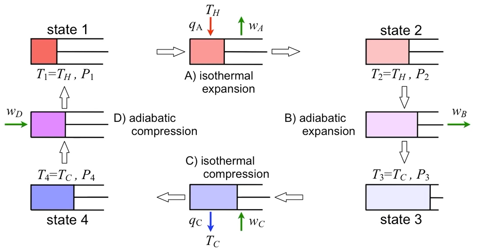
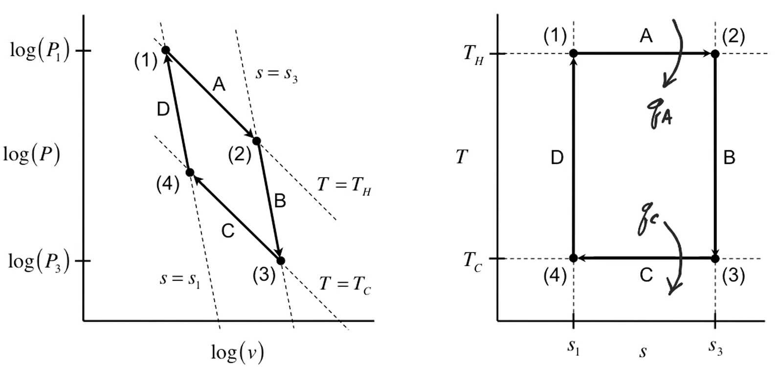
Carnot cycle

Description	Equations
Net work	$-W_{\text{net}} = \vert W_{12} \vert + \vert W_{23} \vert - \vert W_{34} \vert - \vert W_{41} \vert$
Net work and heat	$-W_{\text{net}} = \vert Q_H \vert - \vert Q_C \vert$
Carnot efficiency	$\eta = 1 - \dfrac{T_H}{T_C}$
State properties after cycle	$\Delta u_{\text{cycle}} = 0 \newline \Delta h_{\text{cycle}} = 0 \newline \Delta s_{\text{cycle}} = 0$
Entropy change of surrounding	$\Delta s_{\text{surr}} = 0 = -\dfrac{q_H}{T_H} -\dfrac{q_C}{T_C}$

Open System Balance

Description	Equations
Open system balance	$0 = \dot{m}_1 (\hat{h} + \frac{1}{2}v^2 + gz)_1 - \dot{m}_2 (\hat{h} + \frac{1}{2}v^2 + gz)_2$
Shaft work	$\dot{w}_s = \int v \ dP + \Delta \dot{e}_K + \Delta \dot{e}_P$
Nozzle, diffuser simplifications	$0 = \Delta E_P = \dot{Q} = \dot{W}_s$
Turbine, pump, compressor simplifications	$0 = \Delta E_K = \dot{Q}$
Heat exchanger simplifications	$0 = \Delta E_P = \Delta E_K = \dot{W}_s$
Throttling device simplifications	$0 = \Delta E_P = \Delta E_K = \dot{Q} = \dot{W}_s$

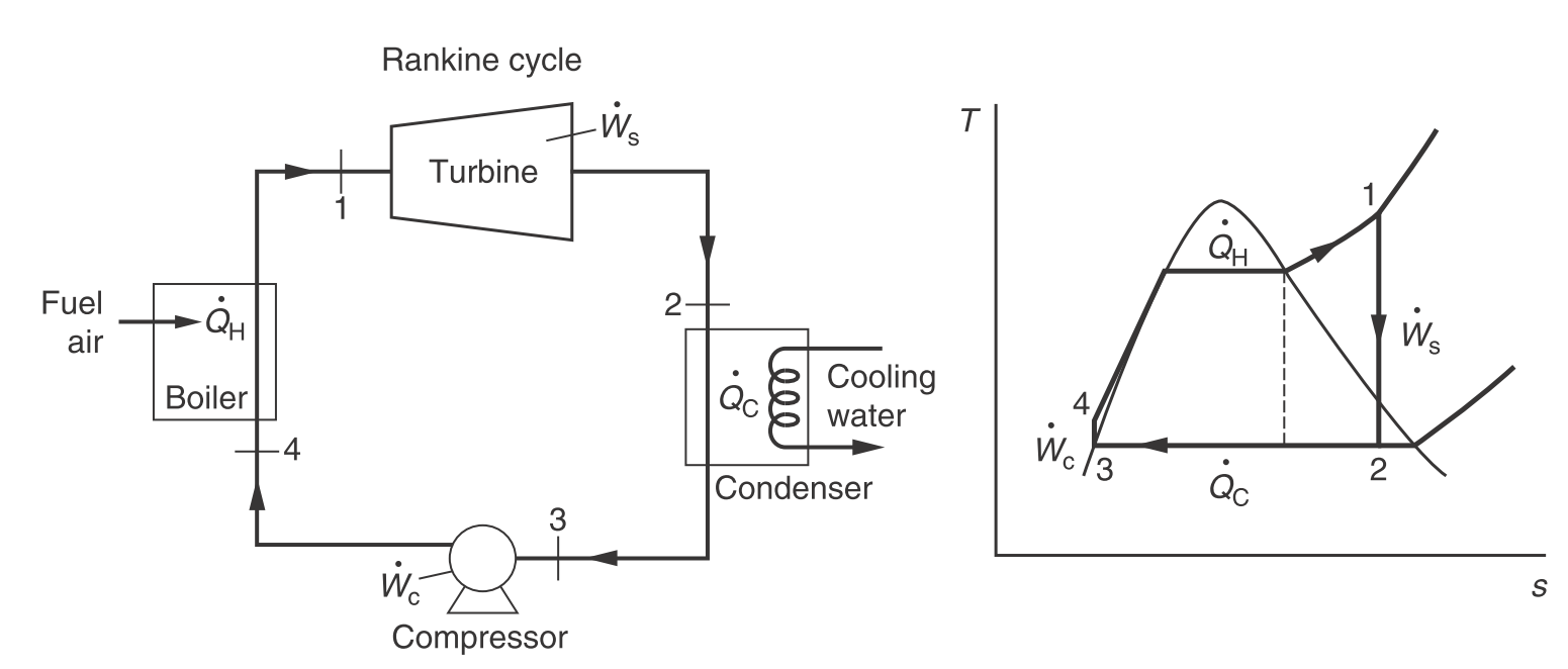
Rankine cycle

Description	Equations
Turbine	$\dot{w}_s = h_2 - h_1 \newline \dot{q} = 0$
Condenser	$\dot{q} = h_3 - h_2 \newline \dot{w}_s = 0$
Compressor	$\dot{w}_c = h_4 - h_3 = v\Delta P \newline \dot{q} = 0$
Boiler	$\dot{q} = h_1 - h_4 \newline \dot{w}_s = 0$
Efficiency	$\eta = \dfrac{\vert\dot{w}_s\vert - \dot{w}_c}{\dot{q}_h} = \dfrac{\vert h_2 - h_1 \vert - (h_4 - h_3)}{h_1 - h_4}$
Net work	$\dot{w}_{\text{net}} = \dot{q}_H - \vert\dot{q}_C\vert = \vert\dot{w}_s\vert - \dot{w}_c$

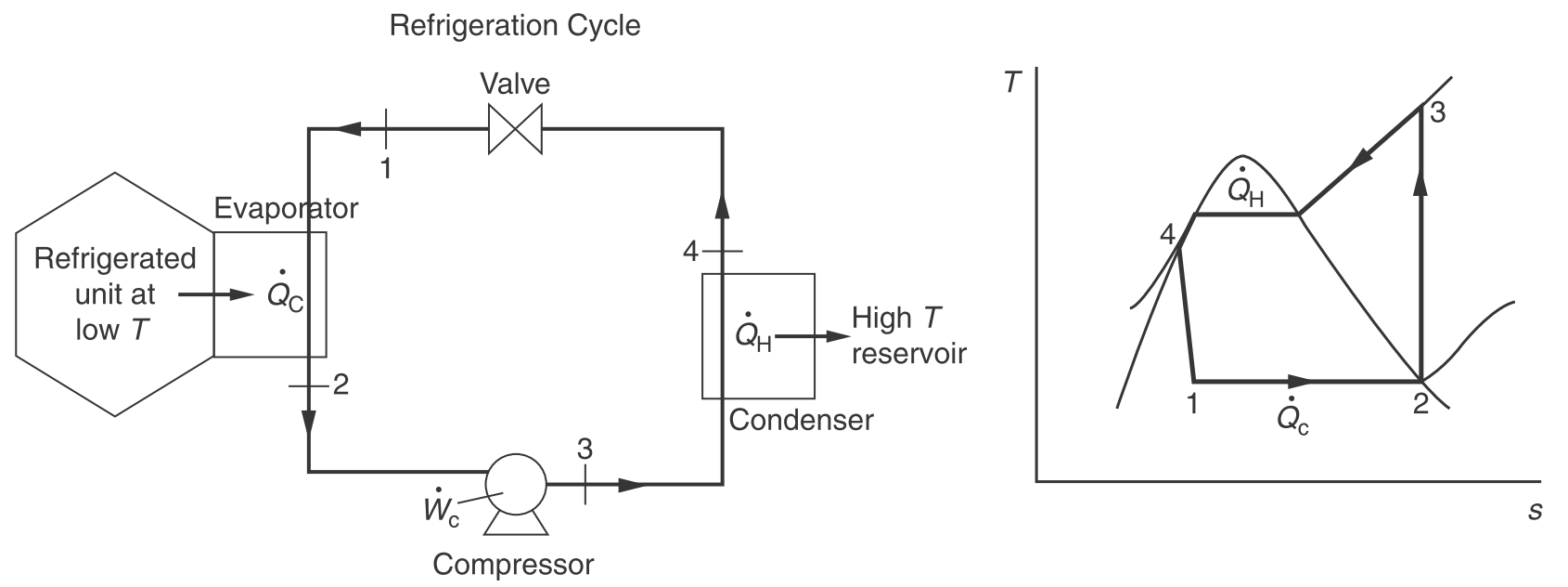
Refrigeration cycle

Description	Equations
Evaporator	$\dot{q} = h_2 - h_1 \newline \dot{w}_s = 0$
Compressor	$\dot{w}_s = h_3 - h_2 \newline \dot{q} = 0$
Condenser	$\dot{q} = h_4 - h_3 \newline \dot{w}_s = 0$
Value	$\dot{w}_s = 0 \newline \dot{q} = 0 \newline \Delta h = 0 \newline \Delta s > 0 \text{ (irreversible expansion)}$
Coefficient of performance	$\mathrm{COP} = \dfrac{\dot{Q}_C}{\dot{W}_c} = \dfrac{h_2 - h_1}{h_3 - h_2}$

Intermolecular Potentials

Description	Equations
Conservative force	$F_{ij} = -\nabla \Gamma_{ij}$
Potential	$\Gamma_{ij} = -\int F_{ij} \ dr$

Attractive potentials (SI unit)

Description	Equations (SI unit)
Coulomb interaction (electrostatic, point charges)	$\Gamma_{ij}(r) = \dfrac{Q_i Q_j}{4\pi\varepsilon_0}\dfrac{1}{r}$
Dipole-dipole interaction (polar, electric dipole, Keesom)	$\Gamma_{ij}(r) = -\dfrac{(2)}{3}\dfrac{\mu_i^2 \mu_j^2}{(4\pi\varepsilon_0)^2}\dfrac{1}{kT}\dfrac{1}{r^6}$
Dipole-induced dipole interaction (induction, Debye)	$\Gamma_{ij}(r) = -\dfrac{\alpha_i \mu_j^2}{(4\pi\varepsilon_0)^2}\dfrac{1}{r^6}$
Induced dipole-induced dipole interaction (dispersion, London)	$\Gamma_{ij}(r) = -\dfrac{3}{2}\dfrac{\alpha_i \alpha_j}{(4\pi\varepsilon_0)^2}\dfrac{I_i I_j}{I_i + I_j}\dfrac{1}{r^6}$

Description	Equations (SI unit)
van der Waals interaction	$\Gamma_{ij}^{\text{vdw}} = \Gamma_{ij}^{\text{K}} + \Gamma_{ij}^{\text{D}} + \Gamma_{ij}^{\text{L}} = -\dfrac{C_{\text{vdw}}}{r^6}$
Keesom coefficient	$C^{\text{K}} = \dfrac{(2)}{3}\dfrac{\mu_i^2 \mu_j^2}{(4\pi\varepsilon_0)^2}\dfrac{1}{kT}$
Debye coefficient	$C^{\text{D}} = \dfrac{\alpha_i \mu_j^2 + \alpha_j \mu_i^2}{(4\pi\varepsilon_0)^2}$
London coefficient	$C^{\text{L}} = \dfrac{3}{2}\dfrac{\alpha_i \alpha_j}{(4\pi\varepsilon_0)^2}\dfrac{I_i I_j}{I_i + I_j}$

Attractive potentials (CGS unit)

Description	Equations (CGS unit)
Coulomb interaction (electrostatic, point charges)	$\Gamma_{ij}(r) = \dfrac{Q_i Q_j}{r}$
Dipole-dipole interaction (polar, electric dipole, Keesom)	$\Gamma_{ij}(r) = -\dfrac{(2)}{3}\dfrac{\mu_i^2 \mu_j^2}{kT}\dfrac{1}{r^6}$
Dipole-induced dipole interaction (induction, Debye)	$\Gamma_{ij}(r) = -\dfrac{\alpha_i \mu_j^2}{r^6}$
Induced dipole-induced dipole interaction (dispersion, London)	$\Gamma_{ij}(r) = -\dfrac{3}{2}\dfrac{\alpha_i \alpha_j}{r^6}\dfrac{I_i I_j}{I_i + I_j}$

Description	Equations (CGS unit)
van der Waals interaction	$\Gamma_{ij}^{\text{vdw}} = \Gamma_{ij}^{\text{K}} + \Gamma_{ij}^{\text{D}} + \Gamma_{ij}^{\text{L}} = -\dfrac{C_{\text{vdw}}}{r^6}$
Keesom coefficient	$C^{\text{K}} = \dfrac{(2)}{3}\dfrac{\mu_i^2 \mu_j^2}{kT}$
Debye coefficient	$C^{\text{D}} = \alpha_i \mu_j^2 + \alpha_j \mu_i^2$
London coefficient	$C^{\text{L}} = \dfrac{3}{2}\alpha_i \alpha_j\dfrac{I_i I_j}{I_i + I_j}$

Repulsive potentials

Description	Equations (SI unit)
Hard sphere model	$\Gamma = \begin{cases} 0 & r > \sigma \\ \infty & r \le \sigma \end{cases}$
Surtherland model	$\Gamma = \begin{cases} -\dfrac{C_{\text{vdw}}}{r^6} & r > \sigma \\ \infty & r \le \sigma \end{cases}$
Lennard-Jones potential	$\Gamma = \dfrac{C_{\text{rep}}}{r^{12}} - \dfrac{C_{\text{vdw}}}{r^6}$
Lennard-Jones potential	$\Gamma = 4\varepsilon \left[ \left(\dfrac{\sigma}{r}\right)^{12} - \left(\dfrac{\sigma}{r}\right)^6 \right]$

Equations of State

Principle of corresponding states

Description	Equations
Ideal gas law	$Pv = RT$
Compressibility factor	$z = \dfrac{Pv}{RT}$
Reduced temperature	$T_r = \dfrac{T}{T_c}$
Reduced pressure	$P_r = \dfrac{P}{P_c}$
Pitzer acentric factor	$\omega = -1 - \log_{10} [P_r^{\text{sat}}(T_r = 0.7)]$
Generalized compressibility	$z = z^{(0)} + \omega z^{(1)}$

Cubic EOS

van der Waals EOS

Description	Equations
van der Waals EOS (pressure explicit form)	$P = \dfrac{RT}{v-b} - \dfrac{a}{v^2}$
van der Waals EOS (cubic form)	$Pv^3 - (RT + Pb)v^2 + av - ab = 0$
van der Waals EOS (reduced form)	$P = \dfrac{8T_r}{3v_r - 1} - \dfrac{3}{v_r^2}$
Intermolecular force (pressure) correction	$a = \dfrac{27}{64}\dfrac{(RT_c)^2}{P_c}$
Volume correction	$b = \dfrac{RT_c}{8P_c}$
Critical compressibility factor	$z_c = \frac{3}{8}$

Redlich-Kwong EOS

Description	Equations
Redlich-Kwong EOS	$P = \dfrac{RT}{v-b} - \dfrac{a}{\sqrt{T}v(v+b)}$
Intermolecular force (pressure) correction	$a = 0.42748 \dfrac{R^2 T_c^{2.5}}{P_c}$
Volume correction	$b = 0.08664 \dfrac{RT_c}{P_c}$
Critical compressibility factor	$z_c = \frac{1}{3}$

Peng-Robinson EOS

Description	Equations
Peng-Robinson EOS	$P = \dfrac{RT}{v-b} - \dfrac{a \alpha(T)}{v(v+b) + b(v-b)}$
Intermolecular force (pressure) correction	$a = 0.45724 \dfrac{R^2 T_c^{2}}{P_c}$
Volume correction	$b = 0.07780 \dfrac{RT_c}{P_c}$
Constant	$\alpha(T) = [1 + \kappa(1 - \sqrt{T_r})]^2$
Constant	$\kappa = 0.37464 + 1.54226\omega - 0.26992\omega^2$
Critical compressibility factor	$z_c = 0.307$

Virial EOS

Description	Equations
Virial EOS	$z = \dfrac{Pv}{RT} = 1 + \dfrac{B}{v} + \dfrac{C}{v^2} + \dfrac{D}{v^3} + \cdots$
Second virial coefficient	$B = \dfrac{RT_c B_r}{P_c}$
Reduced second virial coefficient	$B_r = B^{(0)} + \omega B^{(1)}$
0th order correction	$B^{(0)} = 0.083 - \dfrac{0.422}{T_r^{1.6}}$
1st order correction	$B^{(1)} = 0.139 - \dfrac{0.172}{T_r^{4.2}}$

Mixing rules of EOS parameters

Cubic EOS

Description	Equations
$a$ for binary mixtures	$a_{\text{mix}} = y_1^2 a_1 + 2 y_1y_2 a_{12} + y_2^2 a_2$
$a$ of different species interaction	$a_{12} = \sqrt{a_1 a_2}(1 - k_{12})$
$b$ for binary mixtures	$b_{\text{mix}} = y_1b_1 + y_2b_2$
$a$ for multicomponent mixtures	$a_{\text{mix}} = \sum\limits_i\sum\limits_j y_i y_j a_{ij}$
$b$ for multicomponent mixtures	$b_{\text{mix}} = \sum\limits_i y_i b_{i}$

Virial EOS

Description	Equations
Second virial coefficient for binary mixture	$B_{\text{mix}} = y_1^2 B_{11} + 2 y_1 y_2 B_{12} + y_2^2 B_{22}$
Second virial coefficient for multicomponent mixture	$B_{\text{mix}} = \sum\limits_i\sum\limits_j y_i y_j B_{ij}$
Third virial coefficient for multicomponent mixture	$C_{\text{mix}} = \sum\limits_i\sum\limits_j\sum\limits_k y_i y_j y_k C_{ijk}$

Principle of corresponding state

Description	Equations
Pseudocritical temperature	$T_{pc} = \sum y_i T_{c, i}$
Pseudocritical pressure	$P_{pc} = \sum y_i P_{c, i}$
Pseudocritical acentric factor	$\omega_{pc} = \sum y_i \omega_{c, i}$

EOS for liquids and solids

Description	Equations
Thermal expansion coefficient	$\beta = \dfrac{1}{v} \left(\dfrac{\partial v}{\partial T}\right)_P$
Isothermal compressibility	$\kappa = -\dfrac{1}{v} \left(\dfrac{\partial v}{\partial P}\right)_T$
Rackett equation	$v_l^{\text{sat}} = \dfrac{RT_c}{P_c} (0.29056 - 0.08775 \omega)^{(1 + (1 - T_r)^{2/7})}$

Thermodynamic Relations

Mathematical Relations

Description	Equations
Total differential	$dz = \left(\dfrac{\partial z}{\partial x}\right)_y dx + \left(\dfrac{\partial z}{\partial y}\right)_x dy$
Clairaut’s theorem Symmetry of second derivative	$\dfrac{\partial}{\partial x} \left(\dfrac{\partial z}{\partial y} \right) = \dfrac{\partial}{\partial y} \left( \dfrac{\partial z}{\partial x} \right)$
Chain rule	$\dfrac{\partial z}{\partial x} = \dfrac{\partial z}{\partial y}\dfrac{\partial y}{\partial x}$
Cyclic relation Triple chain rule	$\left(\dfrac{\partial x}{\partial y}\right)_z \left(\dfrac{\partial y}{\partial z}\right)_x \left(\dfrac{\partial z}{\partial x}\right)_y = -1$

Thermodynamic Relations

Relations	Internal energy $u$	Enthalpy $h$	Helmholz energy $a$	Gibbs energy $g$
Definition	-	$h = u + Pv$	$a = u - Ts$	$g = h - Ts$
Fundamental property relations	$du = Tds - Pdv$	$dh = Tds + vdP$	$da = -sdT - Pdv$	$dg = -sdT + vdP$
Fundamental grouping	$\lbrace u, s, v \rbrace$	$\lbrace h, s, P \rbrace$	$\lbrace a, T, v \rbrace$	$\lbrace g, T, P \rbrace$
Fundamental grouping relations	$\left(\frac{\partial u}{\partial s}\right)_v = T$	$\left(\frac{\partial h}{\partial s}\right)_P = T$	$\left(\frac{\partial a}{\partial T}\right)_v = -s$	$\left(\frac{\partial g}{\partial T}\right)_P = -s$
Fundamental grouping relations	$\left(\frac{\partial u}{\partial v}\right)_s = -P$	$\left(\frac{\partial h}{\partial P}\right)_s = v$	$\left(\frac{\partial a}{\partial v}\right)_T = -P$	$\left(\frac{\partial g}{\partial P}\right)_T = v$
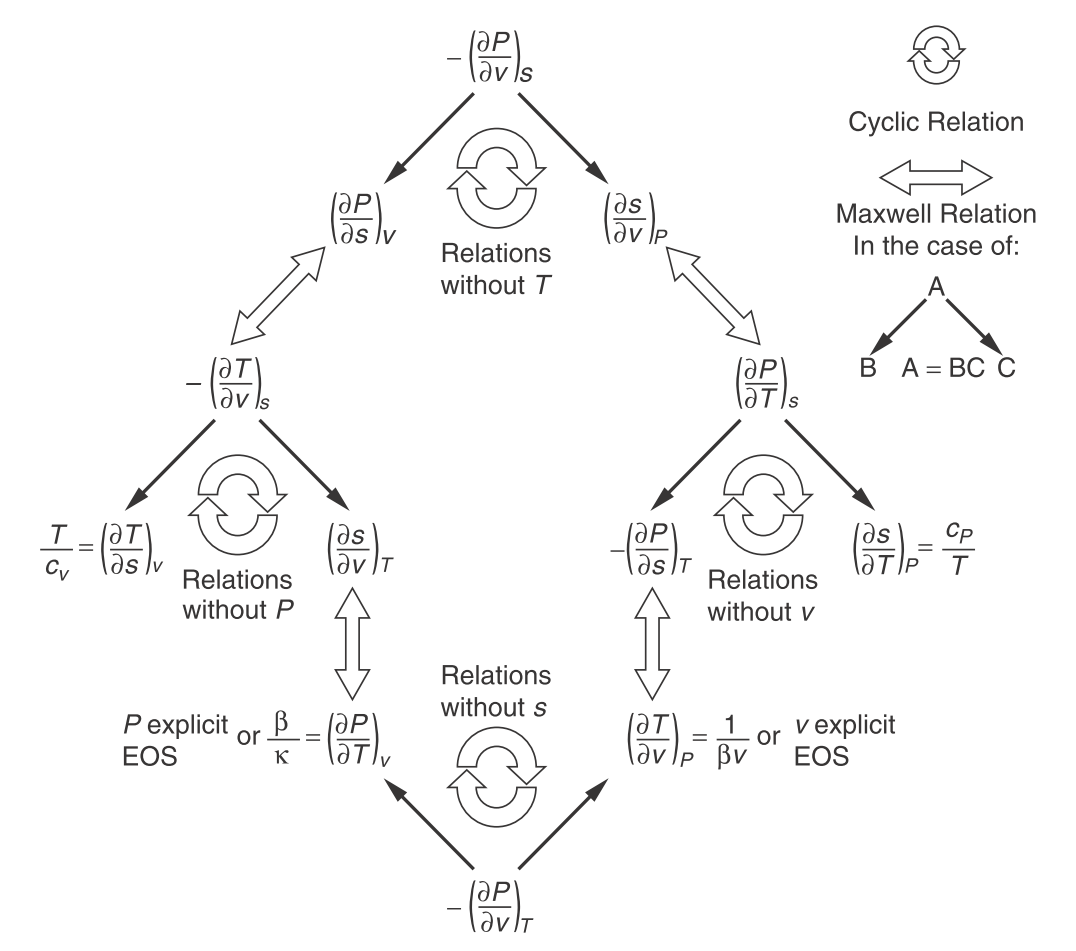
Maxwell’s relations	$\left(\frac{\partial T}{\partial v}\right)_s = -\left(\frac{\partial P}{\partial s}\right)_v$	$\left(\frac{\partial T}{\partial P}\right)_s = \left(\frac{\partial v}{\partial s}\right)_P$	$\left(\frac{\partial s}{\partial v}\right)_T = \left(\frac{\partial P}{\partial T}\right)_v$	$\left(\frac{\partial s}{\partial P}\right)_T = -\left(\frac{\partial v}{\partial T}\right)_P$

Measurable properties

Description	Equations
Constant volume heat capacity	$c_v = \left(\dfrac{\partial u}{\partial T}\right)_v = T \left(\dfrac{\partial s}{\partial T}\right)_v$
Constant pressure heat capacity	$c_P = \left(\dfrac{\partial h}{\partial T}\right)_P = T \left(\dfrac{\partial s}{\partial T}\right)_P$
Constant volume heat capacity of real gas	$c_v^{\text{real}} = c_v^{\text{ideal}} + \displaystyle\int_{v_{\text{ideal}}}^{v_{\text{real}}} \left[T \left(\dfrac{\partial^2 P}{\partial T^2}\right)_v\right] dv$
Constant pressure heat capacity of real gas	$c_P^{\text{real}} = c_P^{\text{ideal}} - \displaystyle\int_{P_{\text{ideal}}}^{P_{\text{real}}} \left[T \left(\dfrac{\partial^2 v}{\partial T^2}\right)_P\right] dP$
Thermal expansion coefficient	$\beta = \dfrac{1}{v} \left(\dfrac{\partial v}{\partial T}\right)_P$
Thermal expansion coefficient of ideal gas	$\beta = \dfrac{1}{T}$
Isothermal compressibility	$\kappa = -\dfrac{1}{v} \left(\dfrac{\partial v}{\partial P}\right)_T$
Isothermal compressibility of ideal gas	$\kappa = \dfrac{1}{P}$

Property changes

Description	Equations
Entropy change $s(T, v)$	$ds = \dfrac{c_v}{T} dT + \left(\dfrac{\partial P}{\partial T}\right)_v dv$
Entropy change $s(T, P)$	$ds = \dfrac{c_P}{T} dT + \left(\dfrac{\partial v}{\partial T}\right)_P dP$
Internal energy change $u(T, v)$	$du = c_v dT + \left[T \left(\dfrac{\partial P}{\partial T}\right)_v - P\right] dv$
Enthalpy change $h(T, P)$	$dh = c_P dT + \left[-T \left(\dfrac{\partial v}{\partial T}\right)_P + v\right] dP$

Property changes $(T, P)$

General $f(T, P)$	Ideal gas $\beta = \frac{1}{T}, \kappa = \frac{1}{P}$
$ds = \dfrac{c_P}{T} dT - \beta v \ dP$	$ds = \dfrac{c_P}{T} dT - \dfrac{R}{P} dP$
$dv = \beta v \ dT - \kappa v \ dP$	$dv = \dfrac{v}{T}dT - \dfrac{v}{P}dP$
$du = (c_P - \beta Pv)dT + (\kappa Pv - \beta vT)dP$	$du = (c_P - R)dT$
$dh = (c_P - \beta Pv)dT + v \ dP$	$dh = c_P \ dT$
$da = -s \ dT + (\kappa Pv - \beta vT)dP$	$da = -s \ dT$
$dg = -s \ dT + v \ dP$	$dg = -s \ dT + v \ dP$

Departure functions

Description	Equations
General departure function	$\mathrm{dep = real - ideal}$
Enthalpy departure function	$\Delta h^{\text{dep}} = h^{\text{real}} - h^{\text{ideal}}$
Entropy departure function	$\Delta s^{\text{dep}} = s^{\text{real}} - s^{\text{ideal}}$
Dimensionless enthalpy departure function	$\dfrac{\Delta h^{\text{dep}}}{RT_c} = T_r^2 \displaystyle\int_0^P \left[-\dfrac{1}{P_r}\left(\dfrac{\partial z}{\partial T_r}\right)_P \right] dP_r$
Dimensionless entropy departure function	$\dfrac{\Delta s^{\text{dep}}}{R} = \displaystyle\int_0^P -\left[\dfrac{z-1}{P_r} + \dfrac{T_r}{P_r}\left(\dfrac{\partial z}{\partial T_r}\right)_P \right] dP_r$
Dimensionless enthalpy departure function with Lee-Kesler EOS	$\dfrac{\Delta h^{\text{dep}}}{RT_c} = \left[\dfrac{\Delta h^{\text{dep}}}{RT_c}\right]^{(0)} + \omega \left[\dfrac{\Delta h^{\text{dep}}}{RT_c}\right]^{(1)}$
Dimensionless entropy departure function with Lee-Kesler EOS	$\dfrac{\Delta s^{\text{dep}}}{R} = \left[\dfrac{\Delta s^{\text{dep}}}{R}\right]^{(0)} + \omega \left[\dfrac{\Delta s^{\text{dep}}}{R}\right]^{(1)}$

Joule-Thomson Expansion

Description	Equations
Joule-Thomson expansion Adiabatic reversible throttling	$\dot{q} = 0 \newline \dot{w}_s = 0 \newline \Delta h = 0$
Joule-Thomson coefficient	$\mu_{\text{JT}} = \left(\dfrac{\partial T}{\partial P}\right)_h$
Joule-Thomson coefficient	$\mu_{\text{JT}} = \dfrac{\left[-T \left(\dfrac{\partial v}{\partial T}\right)_P + v\right]}{c_P^{\text{real}}}$

Phase Equilibria

Single-component equilibrium

Description	Equations
Gibbs free energy	$g = h - Ts$
Second law of thermodynamics	$dG_i \le 0$
Criteria for chemical equilibrium	$g_i^\alpha = g_i^\beta$
Clapeyron equation General phase equilibrium	$\dfrac{dP}{dT} = \dfrac{\Delta s}{\Delta v} = \dfrac{\Delta h}{T\Delta v}$
Clausius-Clapeyron equation ★ Vapor-liquid equilibrium ★ Ideal gas, negligible liquid volume	$\dfrac{dP^{\text{sat}}}{P^{\text{sat}}} = \dfrac{\Delta h_{\text{vap}} dT}{RT^2}$
Clausius-Clapeyron equation ★ Vapor-liquid equilibrium ★ Ideal gas, negligible liquid volume ★ $\Delta h_{\text{vap}}$ independent of $T$	$\ln\dfrac{P_2^{\text{sat}}}{P_1^{\text{sat}}} = -\dfrac{\Delta h_{\text{vap}}}{R} \left(\dfrac{1}{T_2} - \dfrac{1}{T_1}\right)$
Antoine’s equation	$\ln P^{\text{sat}} = A - \dfrac{B}{C+T}$

Properties of mixtures

Description	Equations
Extensive total solution (mixture) property	$K$
Intensive total solution (mixture) property	$k = \dfrac{K}{n}$
Extensive pure species property	$K_i$
Intensive pure species property	$k_i = \dfrac{K_i}{n_i}$
Partial molar property	$\overline{K}_i = \left(\dfrac{\partial K}{\partial n_i}\right)_{T, P, n_{j\not= i}}$
Limiting case of partial molar property	$\displaystyle\lim_{x_i \to 1} \overline{K}_i = k_i \newline \lim_{x_i \to 0} \overline{K}_i = \overline{K}_i^\infty$
Differential of extensive property	$dK = \left(\frac{\partial K}{\partial T}\right)_{P, n_i} dT + \left(\frac{\partial K}{\partial P}\right)_{T, n_i} dP + \sum \overline{K}_i dn_i$
Relation between properties ★ Constant T, P	$K = \sum n_i \overline{K}_i \newline k = \sum x_i \overline{K}_i$
Gibbs-Duhem equation ★ Constant T, P	$\sum n_i d\overline{K}_i = 0$
Corollary of Gibbs-Duhem equation ★ Binary mixture	$x_1 \dfrac{d\overline{K_1}}{d x_1} + x_2 \dfrac{d\overline{K_2}}{d x_1} = 0$

Property changes of mixtures

Description	Equations
Extensive property change of mixing	$\Delta K_{\text{mix}} = K - \sum n_i k_i \newline \Delta K_{\text{mix}} = \sum n_i (\overline{K}_i - k_i)$
Intensive property change of mixing	$\Delta k_{\text{mix}} = k - \sum x_i k_i \newline \Delta k_{\text{mix}} = \sum x_i (\overline{K}_i - k_i)$
Enthalpy of mixing	$\Delta h_{\text{mix}} = \sum x_i (\overline{h}_i - h_i)$
Enthalpy of mixing	$\Delta h_{\text{mix}} = \dfrac{\Delta \tilde{h}_s}{n+1} = \Delta \tilde{h}_s x_1$
Enthalpy of solution	$\Delta \tilde{h}_s = \dfrac{\Delta h_{\text{mix}}}{x_1} = \Delta h_{\text{mix}}(n+1)$
Entropy of mixing ★ Ideal gas, regular solution	$\Delta s_{\text{mix}} = -R\sum y_i \ln y_i$
Partial molar property change of mixing	$\overline{\Delta K}_{\text{mix}, i} = \overline{K}_i - k_i$

Determination of $\overline{G}_i$

Description	Equations
Partial molar volume of species 1 ★ Virial EOS	$\overline{V}_1 = \dfrac{RT}{P} + (y_1^2 + 2y_1 y_2)B_{11} + 2y_2^2 B_{12} - y_2^2 B_{22}$
Partial molar volume of species 2 ★ Virial EOS	$\overline{V}_2 = \dfrac{RT}{P} - y_1^2 B_{11} + 2y_1^2 B_{12} + (y_2^2 + 2y_1 y_2)B_{22}$
Volume change of mixing ★ Virial EOS	$\Delta v_{\text{mix}} = y_1 y_2(2B_{12} - B_{11} - B_{22})$
Partial molar property	$\overline{K}_i = k_i + \overline{\Delta K}_{\text{mix}, i}$
Graphical method Slope is difference	$\dfrac{dk}{dx_1} = \overline{K}_1 - \overline{K}_2$
Graphical method $\overline{K}_2$ is intercept	$k = x_1 \dfrac{dk}{dx_1} + \overline{K}_2$
Graphical method $\overline{K}_2$ explicit	$\overline{K}_2 = k - x_1 \dfrac{dk}{dx_1}$

$T$ and $P$ dependence of $\overline{G}_i$

Description	Equations
Partial molar Gibbs energy dependence on temperature	$\left(\dfrac{\partial \overline{G}_i}{\partial T}\right)_{P, n_i} = -\overline{S}_i$
Partial molar Gibbs energy dependence on temperature (measurable)	$\left[\dfrac{\partial}{\partial T}\left(\dfrac{\overline{G}_i}{T}\right)\right]_{P, n_i} = -\dfrac{\overline{H}_i}{T^2}$
Partial molar Gibbs energy dependence on pressure	$\left(\dfrac{\partial \overline{G}_i}{\partial P}\right)_{T, n_i} = -\overline{V}_i$

Multicomponent equilibrium

Description	Equations
Chemical potential	$\mu_i = \overline{G}_i = \left(\dfrac{\partial G}{\partial n_i}\right)_{T, P, n_{j \not= i}}$
Criteria for chemical equilibrium	$\mu_i^\alpha = \mu_i^\beta$
General multicomponent equilibrium	$\Delta \left[ -\dfrac{\overline{H}_i}{T^2}dT - \dfrac{\overline{V}_i}{T}dP + \dfrac{1}{T} \left[\dfrac{\partial \mu_i}{\partial x_i}\right]_{T, P} dx_i \right] = 0$
Vapor liquid equilibrium ★ Ideal gas	$\begin{aligned} &-\dfrac{h_i^v}{T^2}dT - R\dfrac{dP}{P} + R\dfrac{dx_i^v}{x_i^v} = -\dfrac{\overline{H}_i^l}{T^2}dT - \dfrac{\overline{V}_i^l}{T}dP + \dfrac{1}{T} \left[\dfrac{\partial \mu_i^l}{\partial x_i}\right]_{T, P} dx_i \end{aligned}$

Fugacity

Definition of fugacity

Description	Equations
Definition of fugacity of pure species ★ Constant T	$g_i - g_i^\circ = RT\ln\left(\dfrac{f_i}{f_i^\circ}\right) \newline \lim\limits_{P \to 0} \varphi_i = 1$
Fugacity of pure species ★ Constant T	$f_i = \varphi_i P$
Fugacity coefficient of pure species	$\varphi_i = \dfrac{f_i}{P}$
Definition of fugacity of species i in mixture	$\mu_i - \mu_i^\circ = RT\ln\left(\dfrac{\hat{f}_i}{\hat{f}_i^\circ}\right) \newline \lim\limits_{P \to 0} \hat{\varphi}_i = 1$
Fugacity of species i in mixture	$\hat{f}_i = y_i P \hat{\varphi}_i$
Fugacity coefficient of species i in mixture ★ Constant T	$\hat{\varphi}_i = \dfrac{\hat{f}_i}{p_i} = \dfrac{\hat{f}_i}{y_i P}$
Criteria for chemical equilibrium	$\hat{f}_i^\alpha = \hat{f}_i^\beta$

Fugacity in vapor phase

Single component pure species

Description	Equations
Reference state ★ Ideal gas	$P^\circ = P_{\text{low}} \newline T^\circ = T_{\text{sys}} \newline \hat{f}_i^\circ = P^\circ$
Fugacity of pure species ★ Constant T	$f_i = \varphi_i P$
Fugacity coefficient of pure species	$\varphi_i = \dfrac{f_i}{P}$
Fugacity from experimental data	$f_i^v = P^\circ \exp\left(\dfrac{g_i - g_i^\circ}{RT}\right)$
Fugacity coefficient from experimental data	$\varphi_i = \dfrac{P^\circ}{P} \exp\left(\dfrac{g_i - g_i^\circ}{RT}\right)$
Fugacity from EOS	$RT\ln\left(\dfrac{f_i^v}{P^\circ}\right) = \displaystyle\int_{P^\circ}^P v_i \ dP$
Fugacity coefficient from EOS	$\varphi_i = \dfrac{P^\circ}{P} \exp\left[\dfrac{1}{RT}\displaystyle\int_{P^\circ}^P v_i \ dP\right]$
Fugacity coefficient from vdW EOS	$\ln\varphi_i^v = -\ln\left[\dfrac{(v_i - b)P}{RT}\right] + \dfrac{b}{v_i - b} - \dfrac{2a}{RTv_i}$
Fugacity coefficient from virial form of vdW EOS	$\ln\varphi_i^v = \left(b - \dfrac{a}{RT}\right) \dfrac{P}{RT}$
Fugacity coefficient from generalized correlations	$\ln \varphi_i^v = \displaystyle\int_{P^\circ}^P (z_i - 1) \dfrac{dP}{P}$
Generalized fugacity coefficient with Lee-Kesler EOS	$\log\varphi_i = \log\varphi^{(0)} + \omega \log\varphi^{(1)}$

Multicomponent mixtures

Description	Equations
Reference state ★ Ideal gas	$P^\circ = P_{\text{low}} \newline T^\circ = T_{\text{sys}} \newline n_i^\circ = n_{i, \text{sys}} \newline f_i^\circ = y_i P^\circ \newline V^\circ = \dfrac{nRT}{P^\circ}$
Fugacity of species i in mixture ★ EOS ★ Full i-j interaction	$\hat{f}_i = y_i \hat{\varphi}_i P$
Fugacity of species i in mixture ★ Lewis fugacity rule ★ Same species interaction only, i-i interaction	$\hat{f}_i = y_i \varphi_i P \newline \hat{\varphi}_i = \varphi_i$
Fugacity of species i in mixture ★ Ideal gas, no interaction	$\hat{f}_i = y_i P \newline \hat{\varphi}_i = 1$
Fugacity coefficient of species i in mixture ★ Constant T	$\hat{\varphi}_i = \dfrac{\hat{f}_i}{p_i} = \dfrac{\hat{f}_i}{y_i P}$
Fugacity coefficient from v-explicit EOS	$\hat{\varphi}_i = \dfrac{P^\circ}{P} \exp\left[\dfrac{1}{RT}\displaystyle\int_{P^\circ}^P \overline{V}_i \ dP\right]$
Fugacity coefficient from P-explicit EOS	$\hat{\varphi}_i = \dfrac{P^\circ}{P} \exp\left[-\dfrac{1}{RT}\displaystyle\int_{V^\circ}^V \overline{P}_i \ dV\right]$

Fugacity coefficients from cubic EOS

van der Waals EOS

Description	van der Waals EOS
Pure species i	$\ln \varphi_{i}=\dfrac{b_{i}}{v_{i}-b_{i}}-\ln \left(\dfrac{\left(v_{i}-b_{i}\right) P}{R T}\right)-\dfrac{2 a_{i}}{R T v_{i}}$
Species 1 in a binary mixture	$\ln \hat{\varphi}_{1}=\dfrac{b_{1}}{v-b}-\ln \left(\dfrac{(v-b) P}{R T}\right)-\dfrac{2\left(y_{1} a_{1}+y_{2} a_{12}\right)}{R T v}$
Species i in a mixture	$\ln \hat{\varphi}_{i}=\dfrac{b_{i}}{v-b}-\ln \left(\dfrac{(v-b) P}{R T}\right)-\dfrac{2 \sum\limits_{k=1}^{m} y_{k} a_{i k}}{R T v}$

Redlich-Kwong EOS

Description	Redlich-Kwong EOS
Pure species i	$\begin{aligned}\ln \varphi_{i} =& z_{i}-1-\ln \left(\dfrac{\left(v_{i}-b_{i}\right) P}{R T}\right) \\ &- \dfrac{a_{i}}{b_{i} R T^{1.5}} \ln \left(1+\dfrac{b_{i}}{v_{i}}\right)\end{aligned}$
Species 1 in a binary mixture	$\begin{aligned}\ln \hat{\varphi}_{1} =& \dfrac{b_{1}}{b}(z-1)-\ln \left(\dfrac{(v-b) P}{R T}\right) \\ &+ \dfrac{1}{b R T^{1.5}}\left[\dfrac{a b_{1}}{b}-2\left(y_{1} a_{1}+y_{2} a_{12}\right)\right] \ln \left(1+\dfrac{b}{v}\right)\end{aligned}$
Species i in a mixture	$\begin{aligned}\ln \hat{\varphi}_{i} =& \dfrac{b_{i}}{b}(z-1)-\ln \left(\dfrac{(v-b) P}{R T}\right) \\ &+ \dfrac{1}{b R T^{1.5}}\left[\dfrac{a b_{i}}{b}-2 \sum\limits_{k=1}^{m} y_{k} a_{i k}\right] \ln \left(1+\dfrac{b}{v}\right)\end{aligned}$

Peng-Robinson EOS

Description	Peng-Robinson EOS
Pure species i	$\ln \varphi_{i}= z_{i}-1-\ln \left(\dfrac{\left(v_{i}-b_{i}\right) P}{R T}\right)-\dfrac{(a \alpha)_{i}}{2 \sqrt{2} b_{i} R T} \ln \left[\dfrac{v_{i}+(1+\sqrt{2}) b_{i}}{v_{i}+(1-\sqrt{2}) b_{i}}\right]$
Species 1 in a binary mixture	$\begin{aligned}\ln \hat{\varphi}_{1} =& \dfrac{b_{1}}{b}(z-1)-\ln \left(\dfrac{(v-b) P}{R T}\right) \\ &+ \dfrac{a \alpha}{2 \sqrt{2} b R T}\left[\dfrac{b_{1}}{b}-\dfrac{2}{a \alpha}\left(y_{1}(a \alpha)_{1}+y_{2}(a \alpha)_{12}\right)\right] \ln \left[\dfrac{v+(1+\sqrt{2}) b}{v+(1-\sqrt{2}) b}\right]\end{aligned}$
Species i in a mixture	$\begin{aligned}\ln \hat{\varphi}_{i} =& \dfrac{b_{i}}{b}(z-1)-\ln \left(\dfrac{(v-b) P}{R T}\right) \\ &+ \dfrac{a \alpha}{2 \sqrt{2} b R T}\left[\dfrac{b_{i}}{b}-\dfrac{2}{a \alpha} \sum\limits_{k=1}^{m} y_{k}(a \alpha)_{i k}\right] \ln \left[\dfrac{v+(1+\sqrt{2}) b}{v+(1-\sqrt{2}) b}\right]\end{aligned}$

Mixing rules

Description	Equations
Interaction parameter $a$ for multicomponent mixtures	$a_{\text{mix}} = \sum\sum y_i y_j a_{ij}$
Like attractions	$a_{ii} = a_i$
Unlike attractions	$a_{ij} = \sqrt{a_{ii}a_{jj}}(1 - k_{ij})$
Volume parameter $a$ for multicomponent mixtures	$b_{\text{mix}} = \sum y_i b_{i}$

Property changes of mixing of ideal gas

Description	Equations
Volume change of mixing	$\Delta v_{\text{mix}} = 0$
Enthalpy change of mixing	$\Delta h_{\text{mix}} = 0$
Entropy change of mixing	$\Delta s_{\text{mix}} = -R\sum y_i \ln y_i > 0$
Gibbs energy change of mixing	$\Delta g_{\text{mix}} = RT \sum y_i \ln y_i < 0$

Fugacity in liquid phase

Reference states

Description	Equations
Reference state of fugacity in ideal solution	$\hat{f}_i^\circ = x_i f_i^\circ$
Lewis/Randall rule reference state of fugacity ★ Solvent, pure limit ★ Same species (a-a) interaction only	$f_i^\circ = f_i \newline \hat{f}_i^\circ = x_i f_i$
Henry’s law reference state of fugacity ★ Solute, dilute limit ★ Different species (a-b) interaction only	$f_i^\circ = \mathcal{H}_i \newline \hat{f}_i^\circ = x_i \mathcal{H}_i$

Lewis/Randall rule

Description	Equations
Lewis/Randall rule reference state of fugacity ★ Solvent, pure limit ★ Same species (a-a) interaction only	$f_i^\circ = f_i \newline \hat{f}_i^\circ = x_i f_i$
Pure liquid fugacity with Poynting correction at T, P	$f_i^l = \varphi_i^{\text{sat}} P_i^{\text{sat}} \exp\left[ \displaystyle\int_{P_i^{\text{sat}}}^{P} \dfrac{v_i^l}{RT} dP \right]$
Pure liquid fugacity with Poynting correction at T, P ★ Incompressible liquid	$f_i^l = \varphi_i^{\text{sat}} P_i^{\text{sat}} \exp\left[ \dfrac{v_i^l}{RT} (P - P_i^{\text{sat}}) \right]$
Pure liquid fugacity ★ $P \approx P^{\text{sat}}$	$f_i^l = \varphi_i^{\text{sat}} P_i^{\text{sat}}$
Pure liquid fugacity ★ Ideal gas (low P, low sat P)	$f_i^l = P_i^{\text{sat}}$

Henry’s law

Description	Equations
Henry’s law reference state of fugacity ★ Solute, dilute limit ★ Different species (a-b) interaction only	$f_i^\circ = \mathcal{H}_i \newline \hat{f}_i^\circ = x_i \mathcal{H}_i$
Pressure dependence of Henry’s constant	$\mathcal{H}_i(P) = \mathcal{H}_i(P_1) \exp\left[ \displaystyle\int_{P_0}^{P} \dfrac{\overline{V}_i^\infty}{RT} dP \right]$
Temperature dependence of Henry’s constant	$\mathcal{H}_i(T) = \mathcal{H}_i(T_1) \exp\left[ \displaystyle\int_{T_0}^{T} \dfrac{h_i^v - \overline{H}_i^\infty}{RT^2} dP \right]$

Activity coefficient

Description	Equations
Activity coefficient	$\gamma_i = \dfrac{\hat{f}_i^l}{\hat{f}_i^\circ} = \dfrac{\hat{f}_i^l}{x_i f_i^\circ}$
Activity coefficient in Lewis/Randall rule reference state	$\lim\limits_{x_i \to 0} \gamma_i^{\text{LR}} = \dfrac{\mathcal{H}_i}{f_i} \newline \lim\limits_{x_i \to 1} \gamma_i^{\text{LR}} = 1$
Activity coefficient in Henry’s law reference state	$\lim\limits_{x_i \to 0} \gamma_i^{\text{H}} = 1 \newline \lim\limits_{x_i \to 1} \gamma_i^{\text{H}} = \dfrac{f_i}{\mathcal{H}_i}$
Activity	$a_i = \dfrac{\hat{f}_i^l}{f_i^\circ} \newline a_i = x_i \gamma_i$
Gibbs-Duhem Equation ★ Constant T, P	$\sum x_i d(\ln \gamma_i) = 0$
Corollary of Gibbs-Duhem equation ★ Binary mixture	$x_1 \left(\dfrac{\partial \ln \gamma_1}{\partial x_1}\right)_{T, P} + x_2 \left(\dfrac{\partial \ln \gamma_2}{\partial x_2}\right)_{T, P} = 0$

Excess properties

Description	Equations
Excess property	$k^E = k^{\text{real}} - k^{\text{ideal}}$
Excess property	$k^E = \Delta k_{\text{mix}}^{\text{real}} - \Delta k_{\text{mix}}^{\text{ideal}}$
Partial molar excess property	$\overline{K}_i^E = \overline{K}_i^{\text{real}} - \overline{K}_i^{\text{ideal}}$
Excess Gibbs free energy	$g^E = \Delta g_{\text{mix}} - RT \sum x_i \ln x_i$
Excess Gibbs free energy	$g^E = RT \sum x_i \ln \gamma_i$
Partial molar excess Gibbs free energy	$\overline{G}_i^E = RT \ln \gamma_i$
Area test for thermodynamic consistency ★ Lewis/Randall reference state ★ Constant T, P	$\displaystyle\int_0^1 \ln \left(\dfrac{\gamma_a}{\gamma_b}\right) dx_a = 0$

$\gamma_i$ for binary systems

Two-suffix Margules equation

Description	Equations
Two-suffix Margules equation	$g^E = A x_a x_b$
Activity coefficient	$\overline{G}_i^{E} = RT\ln\gamma_i \newline \overline{G}_a^{E} = A x_b^2 \newline \overline{G}_b^{E} = A x_a^2$

Three-suffix Margules equation

Description	Equations
Three-suffix Margules equation	$g^E = x_{a} x_{b}[A+B(x_{a}-x_{b})]$
Activity coefficient	$\overline{G}_i^{E} = RT\ln\gamma_i \newline \overline{G}_a^{E} = (A+3 B) x_{b}^{2}-4 B x_{b}^{3} \newline \overline{G}_b^{E} = (A-3 B) x_{a}^{2}+4 B x_{a}^{3}$
Three-suffix Margules equation	$g^E = x_{a} x_{b}(A_{ba} x_{a}+A_{ab} x_{b})$
Activity coefficient	$\overline{G}_i^{E} = RT\ln\gamma_i \newline \overline{G}_a^{E} = x_{b}^{2}\left[A_{a b}+2\left(A_{b a}-A_{ab}\right) x_{a}\right] \newline \overline{G}_b^{E} = x_{a}^{2}\left[A_{b a}+2\left(A_{a b}-A_{b a}\right) x_{b}\right]$

van Laar equation

Description	Equations
van Laar equation	$g^E = x_{a} x_{b}\left(\dfrac{A B}{A x_{a}+B x_{b}}\right)$
Activity coefficient	$\overline{G}_i^{E} = RT\ln\gamma_i \newline \overline{G}_a^{E} = A\left(\dfrac{B x_{b}}{A x_{a}+B x_{b}}\right)^{2} \newline \overline{G}_b^{E} = B\left(\dfrac{A x_{a}}{A x_{a}+B x_{b}}\right)^{2}$

Wilson equation

Description	Equations
Wilson equation	$g^E = -R T\left[x_{a} \ln \left(x_{a}+\Lambda_{a b} x_{b}\right) + x_{b} \ln \left(x_{b}+\Lambda_{b a} x_{a}\right)\right]$
Activity coefficient	$\begin{aligned} \overline{G}_i^{E} &= RT\ln\gamma_i \\ \overline{G}_a^{E} &= -R T\left[\ln \left(x_{a}+\Lambda_{ab} x_{b}\right)+x_{b}\left(\dfrac{\Lambda_{b a}}{x_{b}+\Lambda_{ba}x_{a}}-\dfrac{\Lambda_{a b}}{x_{a}+\Lambda_{a b} x_{b}}\right)\right] \\ \overline{G}_b^{E} &= -R T\left[\ln \left(x_{b}+\Lambda_{ba}x_{a}\right)+x_{a}\left(\dfrac{\Lambda_{a b}}{x_{a}+\Lambda_{a b} x_{b}}-\dfrac{\Lambda_{b a}}{x_{b}+\Lambda_{ba}x_{a}}\right)\right] \end{aligned}$
Wilson parameters	$\Lambda_{ab} = \dfrac{v_b}{v_a}\exp\left(-\dfrac{\lambda_{ab}}{RT}\right) \newline \Lambda_{ba} = \dfrac{v_a}{v_b}\exp\left(-\dfrac{\lambda_{ba}}{RT}\right)$

Non-random two-liquid model (NRTL)

Description	Equations
Non-random two-liquid model (NRTL)	$g^E = R T x_{a} x_{b}\left[\dfrac{\tau_{b a} \mathbf{G}_{b a}}{x_{a}+x_{b} \mathbf{G}_{b a}}+\dfrac{\tau_{a b} \mathbf{G}_{a b}}{x_{b}+x_{a} \mathbf{G}_{a b}}\right]$
Activity coefficient	$\overline{G}_i^{E} = RT\ln\gamma_i \newline \overline{G}_a^{E} = R T x_{b}^{2}\left[\dfrac{\tau_{b a} \mathbf{G}_{b a}^{2}}{\left(x_{a}+x_{b} \mathbf{G}_{b a}\right)^{2}}+\dfrac{\tau_{a b} \mathbf{G}_{a b}}{\left(x_{b}+x_{a} \mathbf{G}_{a b}\right)^{2}}\right] \newline \overline{G}_b^{E} = R T x_{a}^{2}\left[\dfrac{\tau_{b a} \mathbf{G}_{b a}}{\left(x_{a}+x_{b} \mathbf{G}_{b a}\right)^{2}}+\dfrac{\tau_{a b} \mathbf{G}_{a b}^{2}}{\left(x_{a}+x_{b} \mathbf{G}_{a b}\right)^{2}}\right]$
NRTL parameters	$\mathbf{G}_{ab} = \exp(-\alpha \tau_{ab}) \newline \mathbf{G}_{ba} = \exp(-\alpha \tau_{ba})$

$\gamma_i$ for multicomponent systems

Two-suffix Margules equation

Description	Equations
Two-suffix Margules equation (ternary system)	$g^E = A_{ab}x_a x_b + A_{ac}x_a x_c + A_{bc}x_b x_c$
Partial excess Gibbs energy of species a	$\overline{G}^E_a = A_{ab}x_b^2 + A_{ac}x_c^2 + (A_{ab} + A_{ac} - A_{bc})x_b x_c$
Partial excess Gibbs energy of species b	$\overline{G}^E_b = A_{ab}x_a^2 + A_{bc}x_c^2 + (A_{ab} + A_{bc} - A_{ac})x_a x_c$
Partial excess Gibbs energy of species c	$\overline{G}^E_c = A_{ac}x_a^2 + A_{bc}x_b^2 + (A_{ac} + A_{bc} - A_{ab})x_a x_b$
Two-suffix Margules equation (multicomponent system)	$g^E = \sum\limits_i \sum\limits_j \dfrac{A_{ij}}{2}x_i x_j$
Two-suffix Margules parameter	$A_{ii} = 0 \newline A_{ij} = A_{ji}$

Wilson equation

Description	Equations
Wilson equation	$\begin{aligned}\ln \gamma_i = 1-\ln \left(\sum\limits_{j=1}^{m} x_{j} \Lambda_{i j}\right)-\sum\limits_{k=1}^{m} \dfrac{x_{k} \Lambda_{k i}}{\ln \left(\sum\limits_{j=1}^{m} x_{j} \Lambda_{k j}\right)}\end{aligned}$
Wilson parameter	$\Lambda_{jj} = 1$

Non-random two-liquid model (NRTL)

Description	Equations
Non-random two-liquid model (NRTL)	$\begin{aligned}\ln \gamma_i = \frac{\sum\limits_{j=1}^{m} \tau_{j i} x_{j} \mathbf{G}_{j i}}{\sum\limits_{l=1}^{m} x_{l} \mathbf{G}_{l i}}+\sum\limits_{j=1}^{m} \frac{x_{j} \mathbf{G}_{i j}}{\sum\limits_{l=1}^{m} x_{l} \mathbf{G}_{l j}}\left(\tau_{i j}-\frac{\sum\limits_{k=1}^{m} \tau_{k j} x_{k} \mathbf{G}_{k j}}{\sum\limits_{l=1}^{m} x_{l} \mathbf{G}_{l j}}\right) \end{aligned}$
NRTL parameters	$\ln \mathbf{G}_{i j}=-\alpha_{i j} \tau_{i j} \newline \tau_{i j}=0 \newline \mathbf{G}_{i j}=1$

Universal quasi-chemical theory (UNIQUAC)

Description	Equations
Universal quasi-chemical theory (UNIQUAC)	$\begin{aligned} \ln\gamma_i = \ln \frac{\Phi_{i}^{*}}{x_{i}}+\frac{z}{2} q_{i} \ln \frac{\theta_{i}}{\Phi_{i}^{*}}+l_{i}+\frac{\Phi_{i}^{*}}{x_{i}} \sum\limits_{j=1}^{m} x_{j} l_{j}+q_{i}^{\prime}\left[1-\sum\limits_{j=1}^{m} \theta_{j}^{\prime} \tau_{j i}-\sum\limits_{j=1}^{m} \frac{\theta_{j}^{\prime} \tau_{i j}}{\sum\limits_{k=1}^{m} \theta_{k}^{\prime} \tau_{k j}}\right] \end{aligned}$
UNIQUAC parameters	$l_{i}=\dfrac{z}{2}\left(r_{i}-q_{i}\right)-\left(r_{i}-1\right) \newline \tau_{j k}=\exp \left(-\dfrac{a_{j k}}{T}\right) \newline \tau_{k k}=1 \newline \Phi_{i}^{*}=\dfrac{x_{i} r_{i}}{\sum\limits_{j=1}^{m} x_{j} r_{j}} \newline \theta_{i}=\dfrac{x_{i} q_{i}}{\sum\limits_{j=1}^{m} x_{j} q_{j}} \newline \theta_{i}^{\prime}=\dfrac{x_{i} q_{i}^{\prime}}{\sum\limits_{j=1}^{m} x_{j} q_{j}^{\prime}}$

$T$ and $P$ dependence of $g^E$

Description	Equations
Excess Gibbs energy dependence on pressure	$\left(\dfrac{\partial g^E}{\partial P}\right)_{T, n_i} = v^E = \Delta v_{\text{mix}}$
Excess Gibbs energy dependence on temperature	$\left[\dfrac{\partial}{\partial T}\left(\dfrac{g^E}{T}\right)\right]_{P, n_i} = -\dfrac{h^E}{T^2} = -\dfrac{\Delta h_{\text{mix}}}{T^2}$
Excess Gibbs energy dependence on temperature ★ Regular solution	$g^E = RT\sum x_i \ln \gamma_i = \text{constant}$
Excess Gibbs energy dependence on temperature ★ Athermal solution	$\dfrac{g^E}{T} = R\sum x_i \ln \gamma_i = \text{constant}$

$T$ and $P$ dependence of $\gamma_i$

Description	Equations
Activity coefficient dependence on pressure	$\left(\dfrac{\partial \ln\gamma_i}{\partial P}\right)_{T, x} = \dfrac{\overline{V}_i - v_i}{RT}$
Activity coefficient dependence on temperature	$\left(\dfrac{\partial \ln\gamma_i}{\partial T}\right)_{P, x} = -\dfrac{\overline{H}_i - h_i}{RT^2}$

Fugacity in solid phase

Description	Equations
Activity coefficient of pure solids	$\Gamma_i = 1$
Fugacity of pure solids	$\hat{f}_i^s = f_i^s$
Fugacity of solid solutions ★ Treat like liquid solution	$\hat{f}_i^s = X_i \Gamma_i f_i^s$

Phase Equilibria Applications

Vapor-liquid equilibrium (VLE)

Description	Equations
General VLE condition	$\begin{aligned} \hat{f}_i^v &= \hat{f}_i^l \\ y_i \hat{\varphi}_i^v P &= x_i \gamma_i^l f_i^\circ \end{aligned}$

Raoult’s law

Description	Equations
Raoult’s law ★ Ideal gas $\hat{\varphi}_i^v = 1$ ★ Ideal solution $\gamma_i^l = 1$ ★ Lewis/Randall ref state $f_i^\circ = f_i = P_i^{\text{sat}}$	$y_i P = x_i P_i^{\text{sat}}$
$K$-value	$K_i = \dfrac{P_i^{\text{sat}}}{P}$
Partial pressure relation of binary system	$\begin{aligned}P &= y_a P + y_b P \\ &= x_a P_a^{\text{sat}} + (1-x_a)P_b^{\text{sat}}\end{aligned}$
Vapor phase composition of binary system	$y_a = \dfrac{x_a P_a^{\text{sat}}}{x_a P_a^{\text{sat}} + (1-x_a)P_b^{\text{sat}}}$
Partial pressure relation of multicomponent system	$\begin{aligned}P &= \textstyle\sum y_i P \\ &= \textstyle\sum x_i P_i^{\text{sat}}\end{aligned}$
Vapor phase composition of multicomponent system	$y_i = \dfrac{x_i P_i^{\text{sat}}}{\sum x_i P_i^{\text{sat}}}$

Nonideal liquid solution

Description	Equations
Nonideal liquid solution ★ Ideal gas $\hat{\varphi}_i^v = 1$ ★ Lewis/Randall ref state $f_i^\circ = f_i = P_i^{\text{sat}}$	$y_i P = x_i \gamma_i P_i^{\text{sat}}$
Partial pressure relation of binary system	$\begin{aligned}P &= y_a P + y_b P \\ &= x_a \gamma_a P_a^{\text{sat}} + (1-x_a) \gamma_b P_b^{\text{sat}}\end{aligned}$
Vapor phase composition of binary system	$y_a = \dfrac{x_a \gamma_a P_a^{\text{sat}}}{x_a \gamma_a P_a^{\text{sat}} + (1-x_a) \gamma_b P_b^{\text{sat}}}$
Partial pressure relation of multicomponent system	$\begin{aligned}P &= \textstyle\sum y_i P \\ &= \textstyle\sum x_i \gamma_i P_i^{\text{sat}}\end{aligned}$
Vapor phase composition of multicomponent system	$y_i = \dfrac{x_i \gamma_i P_i^{\text{sat}}}{\sum x_i \gamma_i P_i^{\text{sat}}}$

Azeotrope

Description	Equations
Azeotrope	$x_i = y_i$
Azeotrope equilibrium consition	$P = \gamma_i P_i^{\text{sat}}$
Activity coefficient from azeotrope	$\gamma_i = \dfrac{P}{P_i^{\text{sat}}}$
Activity coefficient ratio from azeotrope	$\dfrac{\gamma_a}{\gamma_b} = \dfrac{P_b^{\text{sat}}}{P_a^{\text{sat}}}$

Objective function for modeling $\gamma_i$

Description	Equations
Least square objective function based on pressure	$f_P = \sum (P - P_{\text{calc}})_i^2$
Least square objective function based on excess Gibbs energy	$f_{g^E} = \sum (g^E - g^E_{\text{calc}})_i^2$
Least square objective function based on activity coefficient for binary system	$f_\gamma = \sum \left[ \left(\dfrac{\gamma_a - \gamma_a^{\text{calc}}}{\gamma_a}\right)^2 - \left(\dfrac{\gamma_b - \gamma_b^{\text{calc}}}{\gamma_b}\right)^2 \right]_i$

Solubility of gases in liquids

		Ideal gas	Nonideal gas
Ideal liquid	Solute a	$y_a P = x_a \mathcal{H}_a$	$y_a \varphi_a P = x_a \mathcal{H}_a \exp\left[\displaystyle\int_{P_0}^P \dfrac{\overline{V}_a^\infty}{RT} dP\right]$
	Solvent b	$y_b P = x_b P_b^{\text{sat}}$	$y_b \hat{\varphi}_b P = x_b \varphi_b^{\text{sat}} P_b^{\text{sat}} \exp\left[\displaystyle\int_{P_b^{\text{sat}}}^P \dfrac{v_b^l}{RT} dP\right]$
Nonideal liquid	Solute a	$y_a P = x_a \gamma_a^\mathrm{H} \mathcal{H}_a$	$y_a \varphi_a P = x_a \gamma_a^{\mathrm{H}} \mathcal{H}_a \exp\left[\displaystyle\int_{P_0}^P \dfrac{\overline{V}_a^\infty}{RT} dP\right]$
	Solvent b	$\begin{aligned} y_b P = x_b \gamma_b P_b^{\text{sat}} \end{aligned}$	$\begin{aligned} y_b \hat{\varphi}_b P = x_b \gamma_b \varphi_b^{\text{sat}} P_b^{\text{sat}} \exp\left[\displaystyle\int_{P_b^{\text{sat}}}^P \dfrac{v_b^l}{RT} dP\right] \end{aligned}$

Description	Equations
Mixing rule for Henry’s constant	$\ln\mathcal{H}_a = \sum\limits_j x_i \ln\mathcal{H}_{a, j}$

Liquid-liquid equilibrium (LLE)

Description	Equations
General LLE condition	$\begin{aligned}\hat{f}_i^\alpha &= \hat{f}_i^\beta \\ x_i^\alpha \gamma_i^\alpha &= x_i^\beta \gamma_i^\beta \end{aligned}$
Compositions $x_a^\alpha, x_b^\alpha, x_a^\beta, x_b^\beta$ ★ Two-suffix Margules equation	$\begin{aligned} x_a^{\alpha}\exp \left[\dfrac{A}{RT}\left(x_b^{\alpha}\right)^2\right] &= x_a^{\beta}\exp \left[\dfrac{A}{RT}\left(x_b^{\beta}\right)^2\right] \\ x_b^{\alpha}\exp \left[\dfrac{A}{RT}\left(x_a^{\alpha}\right)^2\right] &= x_b^{\beta}\exp \left[\dfrac{A}{RT}\left(x_a^{\beta}\right)^2\right] \\ x_a^\alpha + x_b^\alpha &= 1 \\ x_a^\beta + x_b^\beta &= 1 \end{aligned}$
Genral criteria for instability (separation)	$\left(\dfrac{\partial g^2}{\partial x_a^2}\right)_{T,P} < 0$
Criteria for instability (separation) ★ Two-suffix Margules equation	$\dfrac{RT}{x_ax_b} < 2A$
Upper consolute temperature ★ Two-suffix Margules equation	$T_u = \dfrac{A}{2R}$

Vapor-liquid-liquid equilibrium (VLLE)

Description	Equations
General VLLE condition	$\hat{f}_i^v = \hat{f}_i^\alpha = \hat{f}_i^\beta$
Composition and state variables $x_a^\alpha, x_b^\alpha, x_a^\beta, x_b^\beta, y_a, y_b, T, P$ ★ Two-suffix Margules equation	$\begin{aligned} y_aP = x_a^{\alpha }\exp \left[\frac{A}{RT}\left(x_b^{\alpha }\right)^2\right]P_a^{\text{sat}} &= x_a^{\beta }\exp \left[\frac{A}{RT}\left(x_b^{\beta }\right)^2\right]P_a^{\text{sat}} \\ y_b P = x_b^{\alpha }\exp \left[\frac{A}{RT}\left(x_a^{\alpha }\right)^2\right]P_b^{\text{sat}} &= x_b^{\beta }\exp \left[\frac{A}{RT}\left(x_a^{\beta }\right)^2\right]P_b^{\text{sat}} \\ y_a + y_b &= 1 \\ x_a^\alpha + x_b^\alpha &= 1 \\ x_a^\beta + x_b^\beta &= 1 \end{aligned}$

Solid-liquid equilibrium (SLE), Solid-solid equilibrium (SSE)

Description	Equations
General SLE condition	$\begin{aligned}\hat{f}_i^s &= \hat{f}_i^l \\ X_i \Gamma_i f_i^s &= x_i \gamma_i f_i^l \\ f_s &= x_i \gamma_i f_i^l \end{aligned}$
Composition of SLE ★ Pure solid	$\displaystyle\ln \left[x_i\gamma_i\right]=\frac{\Delta h_{\text{fus},T_m}}{R}\left[\frac{1}{T}-\frac{1}{T_m}\right]-\frac{1}{R}\int_{T_m}^T\frac{\Delta c_P^{sl}}{T}dT+\frac{1}{RT}\int _{T_m}^T\Delta c_P^{sl}dT$
Composition of SLE ★ Pure solid. ★ Constant $\Delta c_P^{sl}$	$\displaystyle\ln \left[x_i\gamma_i\right]=\frac{\Delta h_{\text{fus},T_m}}{R}\left[\frac{1}{T}-\frac{1}{T_m}\right]-\frac{\Delta c_P^{sl}}{R}\left[1-\frac{T_m}{T}-\ln \left(\frac{T}{T_m}\right)\right]$
Composition of SLE ★ Solid solution	$\begin{aligned}\displaystyle\ln \left[\dfrac{x_i\gamma_i}{X_i \Gamma_i}\right]=\frac{\Delta h_{\text{fus},T_m}}{R}\left[\frac{1}{T}-\frac{1}{T_m}\right]-\frac{1}{R}\int_{T_m}^T\frac{\Delta c_P^{sl}}{T}dT+\frac{1}{RT}\int _{T_m}^T\Delta c_P^{sl}dT\end{aligned}$
Composition of SLE ★ Solid solution. ★ Constant $\Delta c_P^{sl}$	$\displaystyle\ln \left[\dfrac{x_i\gamma_i}{X_i \Gamma_i}\right]=\frac{\Delta h_{\text{fus},T_m}}{R}\left[\frac{1}{T}-\frac{1}{T_m}\right]-\frac{\Delta c_P^{sl}}{R}\left[1-\frac{T_m}{T}-\ln \left(\frac{T}{T_m}\right)\right]$

Colligative properties

Description	Equations
Boiling point elevation ★ Solvent $a$, solute $b$	$T-T_{\text{boil}}=\dfrac{RT_{\text{boil}}^2}{\Delta h_{\text{vap}}} \gamma_a x_b$
Activity coefficient from boiling point elevation data	$\gamma_b=\dfrac{\left(T-T_{\text{boil}}\right)\Delta h_{\text{vap}}}{RT_{\text{boil}}^2x_b}$
Freezing point depression ★ Solvent $a$, solute $b$	$T-T_m=\dfrac{RT_m^2}{\Delta h_{\text{fus}}}\gamma_a x_b$
Activity coefficient from freezing point depression data	$\gamma_b=\dfrac{\left(T-T_m\right)\Delta h_{\text{fus}}}{RT_m^2x_b}$
Osmotic pressure	$\Pi =-\dfrac{RT}{v_a}\ln \left(x_a\gamma _a\right)$
Osmotic pressure ★ Ideal solution, dilute $b$	$\Pi =-\dfrac{RT}{v_a}x_b$
Molar mass from osmotic pressure data	$\mathcal{M}_b = \dfrac{RTC_b}{\Pi}$

Chemical Equilibria

Single reaction equilibria

Description	Equations
Chemical reaction expressed in stoichiometric coefficients	$\sum \nu_i A_i$
Extent of reaction	$d\xi = \dfrac{dn_i}{\nu_i}$
Moles of species	$n_i = n_i^\circ + \nu_i \xi$
Chemical equilibrium condition	$\dfrac{dG}{d\xi} = 0 = \sum \mu_i \nu_i$
Gibbs energy of reaction	$\Delta g_{\text{rxn}}^\circ = \sum \nu_i g_i^\circ$
Equilibrium constant	$K = \prod \left(\dfrac{\hat{f}_i}{f_i^\circ}\right)^{\nu_i}$
Equilibrium constant and Gibbs energy of reaction	$\ln K = -\dfrac{\Delta g_{\text{rxn}}^\circ}{RT}$

$K$ dependence on $T$

Description	Equations
Gibbs energy of formation method	$\Delta g_{\text{rxn}}^\circ = \sum \nu_i \Delta g_{f, i}^\circ$
$T$ dependence of $K$	$\dfrac{d}{dT} \ln K = \dfrac{\Delta h_{\text{rxn}}^\circ}{RT^2}$
$T$ dependence of $K$ ★ Constant $\Delta h_{\text{rxn}}^\circ$	$\ln \left(\dfrac{K_1}{K_2}\right)=-\dfrac{\Delta h_{\text{rxn}}^{\circ }}{R}\left(\dfrac{1}{T_2}-\dfrac{1}{T_1}\right)$
$T$ dependence of $K$ ★ $\Delta h_{\text{rxn}}^\circ(T)$	$\ln \left(\dfrac{K_1}{K_2}\right)=-\dfrac{\Delta h_{\text{rxn}}^{\circ }}{R}\left(\dfrac{1}{T_2}-\dfrac{1}{T_1}\right) + \displaystyle\int_{T_1}^{T_2}\dfrac{\int_{T_1}^T\sum\nu_i c_{P,i}dT}{RT^2}dT$

$K$ dependence on concentration

Gas phase reaction

Description	Equations
General expression	$K = \prod \left(\dfrac{y_i \hat{\varphi}_i P}{f_i^\circ}\right)^{\nu_i}$
Lewis fugacity rule	$K = P^\nu \prod \left(y_i \varphi_i\right)^{\nu_i}$
Ideal gas	$K = P^\nu \prod \left(y_i\right)^{\nu_i}$

Liquid phase reaction

Description	Equations
General expression	$K = \prod \left(\dfrac{x_i \gamma_i f_i}{f_i^\circ}\right)^{\nu_i}$
Low pressure, neglegible pressure dependence	$K = P^\nu \prod \left(x_i \gamma_i\right)^{\nu_i}$
Ideal solution	$K = P^\nu \prod \left(x_i\right)^{\nu_i}$

Solid phase reaction

Description	Equations
General expression	$K = \prod \left(\dfrac{X_i \Gamma_i f_i}{f_i^\circ}\right)^{\nu_i}$
Low pressure, neglegible pressure dependence	$K = P^\nu \prod \left(X_i \Gamma_i\right)^{\nu_i}$
Ideal solid solution	$K = P^\nu \prod \left(X_i\right)^{\nu_i}$

Multi-reaction equilibria

Description	Equations
Chemical reactions expressed in stoichiometric coefficients	$\sum\limits_{k=1}^R\sum\limits_{i=1}^m\nu _{k,i}A_i$
Moles of species	$n_i = n_i^\circ + \sum_{k=1}^R \nu_{k, i} \xi$

Electrochemical equilibria

Description	Equations
Gibbs energy and non-Pv work	$\delta W^* \ge (dG)_{T, P}$
Gibbs energy of reaction and reversible work	$W = \Delta G = z\xi FE$
Nerst equation	$E=E_{\text{rxn}}^{\circ }-\dfrac{RT}{zF}\ln \left[\prod\limits_{\text{vap}}(P_i)^{\nu_i} \prod\limits_{\text{liq}}(b_i \gamma_i)^{\nu_i}\right]$
Standard Gibbs energy of reaction	$\Delta g_{\text{rxn}}^{\circ }=-zFE_{\text{rxn}}^{\circ}$
Standard potential of reaction	$E_{\text{rxn}}^{\circ}=-\dfrac{\Delta g_{\text{rxn}}^{\circ }}{zF}$
Standard potential of reaction	$E_{\text{rxn}}^{\circ} = E_{\text{red}}^{\circ}(\text{cathode}) - E_{\text{red}}^{\circ}(\text{anode})$
Average activity coefficient	$\ce{X_a Y_b <=> aX^{(z_+) +} + bY^{(z_-) -}} \newline \gamma_\pm = (\gamma_+^a \gamma_-^b)^{1/(a+b)}$
Average activity coefficient	$\ce{XY <=> X+ + Y-} \newline \gamma_\pm = \sqrt{\gamma_+ \gamma_-}$
Debye-Huckel model	$\ln \gamma_\pm = -A \vert z_+ z_- \vert \sqrt{I}$
Ionic strength	$I = \frac{1}{2}\sum z_i^2 b_i$